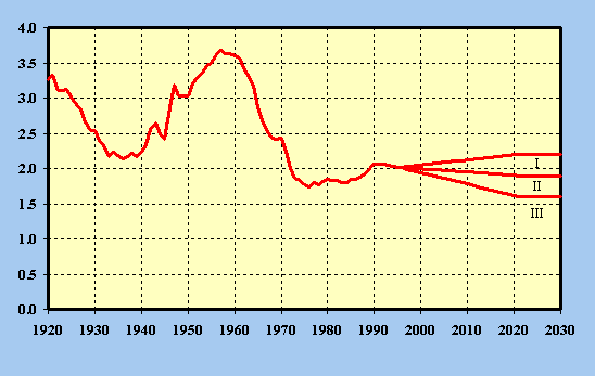
(in children per woman) 1920-2030
Actual and Projected by Alternative
A. Population Size and Growth -- Intermediate Assumption (See table i.)
Under current law, the normal retirement age begins rising in the early 21st century, ultimately reaching age 67. Modifying the aged dependency ratio to reflect the increase in the normal retirement age, the aged dependency ratio for age 66, which becomes the normal retirement age in 2005, is .193. The normal retirement age reaches 67 in 2022. In 2025 the aged dependency ratio is .260 for age 67 compared to .314 for age 65. In 2080 the aged dependency ratio is projected to be .365 for a normal retirement age of 67 and .421 for a normal retirement age of 65.
B. Recent Trends in Population Components
C. Demographic Assumptions - 1997 Trustees Report (See table ii.)
II. Assumptions and Methods
Actuarial estimates of future income and expenditures of the Old-Age and Survivors Insurance and Disability Insurance (OASDI) program are presented every year to the Congress in the Annual Report of the Board of Trustees. These estimates provide fundamental financial guidelines for the policy making process of the OASDI program.
The initial step in the actuarial estimating process is to project the number of people covered by OASDI for each of the next 75 years. This study provides details about the population projections used in preparing the actuarial estimates in the 1997 Annual Report of the OASDI Board of Trustees. These population projections were also used in estimating the future financial status of the Hospital Insurance (HI) program as described in the 1997 Annual Report of the HI Board of Trustees.
The population projections described in this study supersede those published in Actuarial Study Number 110, which were used in the preparation of the 1996 Annual Reports. These new projections start from an estimate of the January 1, 1995 population; reflect more recent data on fertility, mortality, immigration, marriage, and divorce; and revise the projections of mortality, fertility, immigration, divorce, and marriage. Considerably more detailed data than are published here are available from the Office of the Chief Actuary, upon request.
Because eligibility for many categories of OASDI benefits depends on marital status, the population is projected by marital status, as well as by age and sex. The projections start from a recent estimate of the population in the Social Security Area by age, sex, and marital status and from a recent estimate of existing marriages by age of husband and age of wife. Three separate projections, an intermediate, a low cost and a high cost, are developed by analyzing historical data and adopting three different sets of assumptions about future net immigration, birth rates, death rates, marriage rates and divorce rates.
The intermediate projection, designated as alternative II, is based on the set of assumptions that is thought to be the most likely to occur among the three sets presented. The low cost, or optimistic, designated as alternative I, produces the most favorable financial effect for the OASDI program. Similarly, the set of assumptions chosen for the high cost, or pessimistic designated as alternative III, produces the most unfavorable financial effect. The low cost and high cost alternatives are designed to give policy makers a sense of the range of variation in the financial projections that might occur if the intermediate assumptions are not realized.
|
Component | July 1 | |||||
| 1990 | 1991 | 1992 | 1993 | 1994 | 1995 | |
| Residents of the fifty States and D.C. and armed forces overseas |
249,910 |
252,646 |
255,431 |
258,140 |
260,655 |
263,036 |
| Adjustment for net census undercount | 4,697 | 4,732 | 4,771 | 4,875 | 4,898 | 4,994 |
| Civilian residents of Puerto Rico | 3,522 | 3,522 | 3,522 | 3,522 | 3,522 | 3,522 |
| Civilian residents of the Virgin Islands | 102 | 102 | 102 | 102 | 102 | 102 |
| Civilian residents of Guam | 133 | 133 | 133 | 133 | 133 | 133 |
| Civilian residents of American Samoa, Palau, and Northern Mariana Islands |
105 |
105 |
105 |
105 |
105 |
105 |
| Federal civilian employees overseas | 60 | 60 | 60 | 60 | 60 | 60 |
| Dependents of Armed Forces and Federal employees overseas |
460 |
429 |
429 |
429 |
429 |
429 |
| Crew members of merchant vessels | 12 | 12 | 12 | 12 | 12 | 12 |
| Other citizens overseas | 525 | 525 | 525 | 525 | 525 | 525 |
| Total | 259,526 | 262,266 | 265,090 | 267,903 | 270,441 | 272,918 |
The estimates of the number of residents of the fifty States and D.C. and Armed Forces overseas as of the above July 1 dates by sex for single years of age through 84, and for the group aged 85 or older, were obtained from the Bureau of the Census. The adjustment for net census undercount was estimated using postcensal survey data from the Bureau of the Census. The numbers of persons in the other components of the Social Security Area as of the above July 1 dates were estimated by sex for single years of age through 84, and for the group aged 85 or older, from data of varying detail. The numbers of civilian residents of Puerto Rico, the Virgin Islands, Guam, American Samoa, Palau and the Northern Mariana Islands were estimated from data obtained from the Bureau of the Census. The numbers of Federal civilian employees overseas, dependents of these Federal civilian employees, and dependents of Armed Forces overseas were based on estimates used by the Bureau of Census. The number of crew members of merchant vessels was estimated from data obtained from the Maritime Administration. The number of other citizens overseas covered by Social Security was estimated from data supplied by the Department of State. The overlap among the components, believed to be small, was ignored.
The July 1, 1994 and July 1, 1995 Social Security Area population estimates by sex for single years of age through age 84, and for the group aged 85 or older, were then interpolated to obtain the starting population as of January 1, 1995. Data from the Medicare program was used to distribute the starting population aged 85 or older into single years of age. The distribution of the starting population by marital status (never married, currently married, currently widowed, and currently divorced) was estimated by age and sex from data published by the Bureau of the Census in Current Population Reports, Series P-20, No. 478. Table 1 shows this starting population by age group, sex, and marital status.
The distribution of the number of existing marriages in the starting population by age of husband crossed
with age of wife was estimated from data published by the Bureau of the Census in the 1980 Census of
Population, Subject Report on Marital Status No. PC80-2-4C. The 1980 census distribution was adjusted
to represent January 1, 1995 by an iterative proration method designed to assure consistency with the
previously estimated number of marriages by age and sex in the starting population.
Table 2 shows the number of marriages in the starting population by age
group of husband crossed with age group of wife.
C. Analysis and Projection of Components of Population Change
In attempting to estimate net immigration and numbers of births, deaths, marriages, and divorces in future years, it is instructive to review and analyze historical trends. Since the actual numbers of births, deaths, marriages, and divorces depend on the size of the population, it is better to analyze them as rates rather than as absolute numbers. A rate is defined as the ratio of the number of occurrences of an event during a year to the midyear population having the potential to experience the event. Because death rates vary significantly by sex, they are calculated for males and females separately. Because rates of birth, death, marriage, and divorce vary greatly by age, they are calculated on an age-specific basis (each age or age group separately) rather than on a crude basis (all ages combined).
Although calculating the rates on an age-specific basis improves accuracy, it also yields a vast number
of figures for each year. Thus, to study trends through time, it becomes helpful, if not necessary, to use
a single statistic that summarizes the age-specific rates for each year. A summarizing statistic is
described in this section for each component of population change.
1. Fertility
Age-specific birth rates are defined as the births during the year to mothers at the specified age divided
by the midyear female population at that age. Birth rates for women at each age 14 through 49 were
obtained from the National Center for Health Statistics for each year 1917 through 1994. To summarize
the fertility experience for a single year, total fertility rates were used. The total fertility rate is a simple
sum of the age-specific birth rates applicable during the year. Thus the total fertility rate can be
interpreted as the number of children that would be born to a woman if she were to survive her
childbearing years and were to experience those age-specific birth rates throughout her childbearing
years. Table 3 give past and projected total fertility rates by alternative.
As a first step in projecting fertility, it is instructive to examine the recent history of fertility in the
United States. During the period 1917 to 1925, the total fertility rate was more than three children per
woman. During the period 1924 to 1933 the total fertility rate declined from 3.1 children per woman to
2.2, and then remained level at 2.1 to 2.2 children per woman through 1940. After 1940, the total
fertility rate once again began to rise, reaching a peak of 3.7 in 1957. This period of high fertility was
followed by a period of declining fertility, reaching a low of 1.74 in 1976. In one decade, from 1962 to
1972, the total fertility rate declined from 3.4 to 2.0 children per woman. The total fertility rate was
fairly stable at 1.8 children per woman until 1987, when it started to increase, reaching a high of 2.07 in
1990. The total fertility rate remained stable through 1992, decreasing slightly to 2.04 in 1993 and
1994. The estimated total fertility rate, based on preliminary data, for 1995 is 2.02. Figure 1 shows the
total fertility rate historically and by alternative.
|
Figure 1. - Total Fertility Rate
(in children per woman) 1920-2030 Actual and Projected by Alternative |
|
|
| Calendar Year |
On average, the ultimate intermediate total fertility rate is expected to be 1.9. The total fertility rate is not expected to return to the high levels of the 1940's, the 1950's, and early 1960's. Several changes in our society have occurred during the past 20 years which have contributed to reducing the number of children being born. Some of these changes are increased availability and use of birth control methods, increased female participation in the labor force, increased prevalence of divorce, increased postponement of marriage and childbearing among young women, and the shift in the perception of the status of children within their families from economic assets to economic liabilities. No significant reversal of these changes is anticipated.
The increase in the total fertility rate for the United States between 1976 and 1990 is largely the result of increases in birth rates among women in their 30s who put off having children when they were in the 20s. Birthrates for women under 30 were fairly stable for the 1976 through 1990 period. Data for 1991 through 1995 indicates a stabilization of the birth rates for women in their 30s and a slight decline for women under 30.
The latest birth expectation survey published by the Bureau of the Census in the Current Population Reports, Series P-20, No. 454, shows birth expectations in the neighborhood of 2.0 to 2.1 children per woman. However, when comparing past birth expectation surveys with actual experience, birth expectations have tended to be higher than the actual number of births. Single women and childless married women who were surveyed have consistently had fewer births than they expected (see, "Assessing Birth Expectations from Current Population Survey: 1971-1981" by Martin O'Connell and Carolyn Rogers in Demography, August, 1983). Taking into account all these factors, an ultimate total fertility rate of 1.9 children per woman was selected as the intermediate assumption for the 1997 report.
To help in selecting ultimate rates for the low cost and high cost alternatives, an examination of the recent total fertility rates in other nations is useful. A comparison of the total fertility rates for the most recent calendar year, as published in the 1994 United Nations Demographic Yearbook, for the U.S., Canada, and nineteen industrialized countries revealed a range of 2.1 in New Zealand to 1.3 in Italy, Greece and Spain. While rates as high as 2.7 children per woman have been recorded over the past decade (Ireland, 1983), the highest rates these countries are currently experiencing range from 2.0 to 2.1, with the U. S. currently at 2.0. At or just below the 1.9 total fertility rate selected as the intermediate assumption are Australia, Canada, Finland, France, Norway and the United Kingdom. For reasons already cited, we do not believe that the total fertility rate for the U.S. will return to a level as high as 2.5 for any sustained period, and have selected 2.2 as the optimistic, low cost assumption. New Zealand was the only country to have a total fertility rate at or above 2.2. Austria, Belgium, Greece, Italy, Japan, Portugal, Spain, and West Germany, had total fertility rates under 1.6. Therefore, it is plausible that the total fertility rate could be as low as 1.6 children per woman over a long period of time. Thus, we have selected 1.6 as the pessimistic, high cost assumption. The ultimate total fertility rate for each alternative was assumed to be first reached in calendar year 2021. The ultimate values selected for the 1997 Trustees Report are lower than those used by the Bureau of the Census in its latest series of population projections, published in Current Population Reports, Series P-25, No. 1130. The Bureau of the Census used a range of 1.91 to 2.58, with an intermediate assumption of 2.25.
Total fertility rates for 1995 and 1996 were estimated from provisional data published by the National
Center for Health Statistics in Monthly Vital Statistics Reports, Volumes 44 and 45. Between 1997 and
2021, the age-specific birth rates were projected separately for each cohort of women such that the
completed cohort fertility rate would gradually approach the assumed ultimate total fertility rate. The
1996 Trustees Report based the relative distribution of age-specified birth rates on the average historical
age distribution attained from all available (42 years of data) prior completed cohort rates. For the 1997
Trustees Report, the average historical age distribution was modified to include only the latest 31
historical completed cohort rates. This methodological change serves to make the relative age
distribution for birth rates more similar to recent data. Table 4 gives the assumed age-specific birth rates
by alternative for selected calendar years.
2. Mortality
Death rates (generally referred to as central death rates) are defined as the number of deaths during the
year divided by the midyear population. These rates were calculated by sex on an age-specific basis for
each year 1900 through 1994. To summarize the mortality experience of a single year and to control for
changes in the age distribution of the population from year to year, age-adjusted death rates (as shown in
table 5) were calculated as a weighted average of the age-specific death rates. The weights used were
the numbers of people in the corresponding age groups of the 1990 U.S. census resident population.
Thus, if the age-adjusted death rate for a particular year and sex is multiplied by the 1990 U.S. census
resident population, the result gives the number of deaths that would have occurred in 1990 for the U.S.
census resident population if the age-specific death rates for that particular year and sex had been
experienced. The age-adjusted death rate is, therefore, equivalent to the crude death rate that would
have been experienced in the 1990 U.S. census resident population.
Age-sex-adjusted death rates are often calculated when one is interested in
summarizing death rates for both sexes combined.
Age-sex-adjusted death rates (shown in table 5) were calculated as a weighted average of the age-sex-specific
death rates, where each weight was the number of people in the corresponding age and sex group of the
1990 U.S. census resident population.
The calculations of adjusted death rates for the 1997 Trustees Report used the 1990 U.S. resident census
population as the standard population, the population providing the weights. The 1996 Trustees Report
used the 1980 census resident population as the standard. As a result of the change in the standard
population, from 1980 to 1990, the death rates differ from Actuarial Study 110 over the historical period
as well as for the projected period.
An examination of the age-adjusted death rates since 1900 reveals several distinct periods of mortality
reduction. During the period 1900 to 1936, annual mortality reduction averaged about 0.8 percent for
males and 0.9 percent for females. Following this was a period of rapid reduction, 1936 to 1954, in
which mortality decreased an average of 1.6 percent per year for males and 2.5 percent for females. The
period 1954 to 1968 saw an actual increase for males of 0.2 percent per year and a much slower
reduction of 0.8 percent per year for females. From 1968 through 1982 rapid reduction in mortality
resumed, averaging 1.8 percent for males and 2.2 percent for females, annually. From 1982 to 1994,
slower reduction in mortality resumed, decreasing an average of 0.8 percent for males and 0.5 percent
for females. These rates of reduction are shown in the following table by sex and age group.
| Historical Average
Annual Percentage Reductions in Age-Adjusted Central Death Rates | ||||||
| Age and sex | 1900-36 | 1936-54 | 1954-68 | 1968-82 | 1982-94 | 1900-94 |
| Male : | ||||||
| 0-14 | 2.91 | 4.75 | 1.66 | 4.39 | 2.60 | 3.26 |
| 15-64 | 1.02 | 1.91 | -.20 | 2.22 | .61 | 1.14 |
| 65-84 | .20 | 1.15 | -.13 | 1.47 | 1.21 | .65 |
| 85+ | .22 | 1.21 | -.89 | 1.56 | -.34 | .38 |
| 65+ | .20 | 1.16 | -.33 | 1.49 | .79 | .58 |
| Total | .78 | 1.60 | -.21 | 1.78 | .78 | .94 |
| Female : | ||||||
| 0-14 | 3.12 | 5.01 | 1.72 | 4.19 | 2.49 | 3.36 |
| 15-64 | 1.19 | 3.62 | .57 | 2.20 | .70 | 1.66 |
| 65-84 | .36 | 2.06 | 1.07 | 2.01 | .58 | 1.07 |
| 85+ | .23 | 1.21 | .13 | 2.06 | .09 | .66 |
| 65+ | .32 | 1.82 | .77 | 2.03 | .42 | .95 |
| Total | .90 | 2.47 | .77 | 2.15 | .54 | 1.33 |
Past reduction in mortality has varied greatly by cause of death. Because it is expected that future reduction in mortality rates will also vary greatly by cause of death, death rates for the years 1968 through 1994 were calculated and analyzed by age group and sex for ten groups of causes of death (based on the Ninth Revision of the International List of Diseases and Causes of Death code numbers). These groups of causes of death are as follows:
| I. | Diseases of the Heart | (390-398, 402, 404-429) |
| II. | Malignant Neoplasms | (140-208) |
| III. | Vascular Diseases | (400-401, 403, 430-459, 582-583, 587) |
| IV. | Accidents, Suicide, and Homicide | (E800-E989) |
| V. | Diseases of the Respiratory System | (460-519) |
| VI. | Congenital Malformations, Diseases of Early Infancy | (740-779) |
| VII. | Diseases of the Digestive System | (520-570, 572-579) |
| VIII. | Diabetes Mellitus | (250) |
| IX. | Cirrhosis of the Liver | (571) |
| X. | All Other Causes excluding AIDS | (042-044) |
For the years 1968 through 1994, death rates for ages under 65 by age group, sex, and cause of death were calculated using the numbers of deaths as tabulated in Vital Statistics of the United States and using the latest census estimates of the resident population as published in the P-25 Series of Current Population Reports. For the years 1968 through 1978, an adjustment was made to the distribution of the numbers of deaths among the ten causes. This adjustment was needed in order to reflect the revision in the cause of death coding that occurred in 1979, thereby making the data for the years 1968 through 1978 more comparable with the coding used for the years 1979 and later. The adjustments were based on comparability ratios published by the National Center for Health Statistics in Monthly Vital Statistics Report, Volume 28, Number 11.
For the ages 65 and over, records of the Medicare program were used to determine rates by age and sex. The numbers of deaths by cause in Vital Statistics of the United States were used to distribute the age-sex specific death rates for ages over 65 into age-sex-cause specific death rates. A detailed analysis of Medicare mortality statistics and a comparison to the statistics provided by the National Center for Health Statistics is contained in "Recent Trends in the Mortality of the Aged" by John C. Wilkin in the Transactions of the Society of Actuaries, Volume XXXIII, 1981.
Average annual reductions in mortality were determined for the period 1968 through 1994 by age group, sex, and cause of death. The values, shown in table 6, were calculated as the complement of the exponential of the slope of the least-squares line through the logarithms of the death rates. The sharpest reductions were in the categories of Congenital Malformations and Diseases of Early Infancy and Vascular Disease, averaging 3.9 and 4.0 percent, respectively, per year. Averaging 2 to 2.5 percent average reduction per year, were Heart Diseases and Cirrhosis of the Liver. Violence averaged 1.8 percent reduction per year, Diabetes Mellitus .6 percent, and Digestive Diseases 1.0 percent reduction per year. The categories of Cancer and of Respiratory Disease and the residual group of other Causes (excluding AIDS) averaged an increase of about 0.5 to 1.3 percent per year.
Future reductions in mortality will depend upon such factors as the development and application of new diagnostic, surgical, and life-sustaining techniques, the presence of environmental pollutants, improvements in exercise and nutrition, the incidence of violence, the isolation and treatment of causes of disease, the emergence of new forms of disease, improvements in prenatal care, the prevalence of cigarette smoking, the misuse of drugs (including alcohol), the extent to which people assume responsibility for their own health, and changes in our conception of the value of life. After considering how these and other factors might affect mortality, we postulated three alternative sets of ultimate annual percentage reductions in death rates by sex, age group, and cause of death for the years after 2020. The age groups for which specific rates of reduction have been selected are: under age 15, 15-64, and 65-84, and 85 and older. These ultimate annual percentage reductions are as follows:
|
Assumed Ultimate Annual Percentage Reductions in Death Rates by Alternative, Sex, Age Group, and Causes | ||||||||||
| Cause of death | ||||||||||
| Alternative, sex, and age group | Heart disease | Cancer | Vascular disease | Violence | Respiratory disease | Infancy | Digestive disease | Diabetes mellitus | Cirrhosis (liver) | Other |
| Male Low Cost alternative: | ||||||||||
| < 15 | 0.3 | 0.8 | 0.3 | 0.6 | 1.4 | 2.9 | 1.2 | 1.1 | 0.8 | 0.2 |
| 15-64 | 0.7 | 0.1 | 1.0 | 0.3 | 0.2 | 1.5 | 1.1 | 0.2 | 1.0 | 0.0 |
| 65-84 | 0.5 | 0.0 | 0.8 | 0.3 | 0.0 | 1.6 | 0.2 | 0.3 | 0.1 | 0.0 |
| 85 + | 0.5 | 0.0 | 0.8 | 0.3 | 0.0 | 1.6 | 0.2 | 0.3 | 0.1 | 0.0 |
| Female Low Cost alternative: | ||||||||||
| < 15 | 0.3 | 0.8 | 0.3 | 0.6 | 1.4 | 2.9 | 1.2 | 1.1 | 0.8 | 0.2 |
| 15-64 | 0.7 | 0.1 | 1.0 | 0.3 | 0.2 | 1.5 | 1.1 | 0.2 | 0.8 | 0.0 |
| 65-84 | 0.5 | 0.0 | 0.8 | 0.3 | 0.0 | 1.6 | 0.2 | 0.3 | 0.1 | 0.0 |
| 85 + | 0.5 | 0.0 | 0.8 | 0.3 | 0.0 | 1.6 | 0.2 | 0.3 | 0.1 | 0.0 |
| Male Intermediate alternative: | ||||||||||
| < 15 | 0.6 | 2.0 | 0.6 | 0.9 | 2.4 | 2.2 | 1.6 | 1.8 | 1.4 | 0.5 |
| 15-64 | 1.5 | 0.3 | 1.8 | 0.5 | 0.3 | 1.1 | 1.6 | 0.3 | 1.5 | 0.3 |
| 65-84 | 1.2 | 0.2 | 1.7 | 0.6 | 0.2 | 1.1 | 0.4 | 0.6 | 0.2 | 0.2 |
| 85 + | 1.1 | 0.2 | 1.7 | 0.6 | 0.2 | 1.1 | 0.4 | 0.6 | 0.2 | 0.2 |
| Female Intermediate alternative: | ||||||||||
| < 15 | 0.6 | 2.0 | 0.6 | 0.9 | 2.4 | 2.2 | 1.6 | 1.8 | 1.4 | 0.5 |
| 15-64 | 1.5 | 0.3 | 1.8 | 0.5 | 0.3 | 1.1 | 1.6 | 0.3 | 1.5 | 0.3 |
| 65-84 | 1.2 | 0.2 | 1.7 | 0.8 | 0.2 | 1.1 | 0.4 | 0.6 | 0.2 | 0.2 |
| 85 + | 1.1 | 0.2 | 1.7 | 0.8 | 0.2 | 1.1 | 0.4 | 0.6 | 0.2 | 0.2 |
| Male High Cost alternative: | ||||||||||
| < 15 | 1.4 | 5.2 | 0.7 | 1.2 | 2.9 | 1.2 | 2.0 | 2.3 | 2.2 | 1.0 |
| 15-64 | 2.0 | 1.2 | 2.1 | 1.0 | 0.5 | 0.5 | 2.4 | 0.4 | 3.0 | 0.6 |
| 65-84 | 1.5 | 1.1 | 2.0 | 1.0 | 0.4 | 0.4 | 0.8 | 0.9 | 0.6 | 0.4 |
| 85 + | 1.3 | 1.1 | 2.0 | 1.0 | 0.4 | 0.4 | 0.8 | 0.9 | 0.6 | 0.4 |
| Female High Cost alternative: | ||||||||||
| < 15 | 1.4 | 5.2 | 0.7 | 1.2 | 2.9 | 1.2 | 2.0 | 2.3 | 2.2 | 1.0 |
| 15-64 | 2.0 | 1.3 | 2.1 | 1.0 | 0.5 | 0.5 | 2.4 | 0.4 | 2.6 | 0.6 |
| 65-84 | 1.6 | 1.2 | 2.0 | 1.1 | 0.4 | 0.4 | 0.8 | 0.9 | 0.6 | 0.4 |
| 85 + | 1.3 | 1.2 | 2.0 | 1.1 | 0.4 | 0.4 | 0.8 | 0.9 | 0.6 | 0.4 |
The annual percentage reductions in the table above are greatest for the high cost alternative and smallest for the low cost alternative, with the exception of the ultimate reductions assumed due to Congenital Malformations and Diseases of Early Infancy. For this cause-of-death group, the low cost alternative reductions are greatest and the high cost alternative reductions are smallest because most of the deaths due to this cause of death occur to those under 5 years of age. Thus, unlike the other causes of death, higher death rates for this cause of death would produce an unfavorable financial effect.
Due to the nature of AIDS, this disease was treated as a separate and special cause of death and death rates due to AIDS were projected by a different method. Although much has been learned about AIDS during the last few years, many uncertainties exist about the future course of this disease. For historical years beginning in 1981 through projected years ending with 1994, central death rates due to AIDS were projected based on numbers of deaths due to AIDS as estimated by the Center for Disease Control. Among the three alternatives, the death rates assumed for the high cost alternative were the greatest and those assumed for the low cost alternative were the smallest. Higher death rates for AIDS result in more cost to the OASDI program. Under the intermediate and high cost alternatives, the central death rates due to AIDS are assumed to reach their peak value around the year 2000. During the next ten years, death rates due to AIDS are assumed to decline rather rapidly as a result of changes in behavior. Thereafter, the rates are assumed to remain relatively constant throughout the remainder of the projection period. For the low cost alternative, the peak in central death rates due to AIDS is assumed to have been reached around 1990, with the projected rates decreasing and stabilizing immediately.
Rapid reductions in infant mortality are expected to continue in the future. However, for the total group younger than 65, future reductions are projected to be relatively small compared with past reductions because very little additional reduction in death rates from infectious diseases (such as poliomyelitis and influenza) is possible and because only a small reduction in mortality from violent causes (accidents, suicide, and homicide) is expected. Reductions for the aged are expected to continue at a relatively rapid pace, as further advances are made against degenerative diseases (such as heart and vascular disease). The gap between male and female mortality is expected to stabilize as women become increasingly subject to many of the same environmental hazards and social pressures as men. Analysis of the period from 1982 through 1994 shows that the female rate of reduction is less than the male rate of reduction. For time periods in this century prior to 1982, mortality reduction was generally greater for females than males.
After adjustment for changes in the age and sex distribution of the population, the intermediate alternative mortality is projected to decrease at an average rate of 0.56 percent per year during the period 1994 through 2071, about half the average annual reduction observed during 1900 through 1994, but greater than the female rate of reduction for the 1982 through 1994 period. During the period 1994 through 2071, the low cost alternative mortality is projected to decrease at a rate about one-sixth the average rate observed during 1900 through 1994, while for the high cost alternative mortality, the projected rate of reduction is about the same as for 1900 through 1994.
The base year for the mortality projections is 1995. Death rates for ages under 65 in 1995 were estimated from provisional data published in Monthly Vital Statistics Reports, Volumes 44. However, instead of using these estimated provisional death rates as the starting point from which mortality projections are made, we use a set of mortality rates calculated to be consistent with the trend inherent in the last 12 years of available data, including the preliminary data, calendar years 1984 through 1995.
For years after 1995, death rates were projected by age group, sex, and cause of death by applying annual percentage reductions (except for the cause of death category of AIDS) to the estimated or projected prior year death rates. The annual reductions that were applied to obtain the 1996 levels were 50 percent for the low cost alternative, 100 percent for the intermediate alternative, and 150 percent for the high cost alternative of the average annual reductions during 1968 through 1994 period. The annual reductions that were assumed to apply to obtain rates for 1997 through 2021 were calculated by a logarithmic formula designed to gradually transform the reductions applied to obtain the 1995 levels into the postulated ultimate annual reductions. The ultimate reductions were assumed to apply during the 2021 through 2080 period. The average annual reductions for the "All Other" category for age 0 were calculated using the period 1974 through 1994, rather than 1968 through 1994 because a distinct shift occurred in 1974, making earlier data inappropriate for this category. Tables 7a-d gives the resulting death rates by age group, sex, and alternative for selected years. Table 7a presents historical death rates for selected calendar years 1990-1995, table 7b presents projected death rates under the 1997 Trustees Report Low Cost alternative for calendar years 2000-2080, table 7c presents the Intermediate alternative, and table 7d the High Cost alternative.
A complete projection of age-sex-specific death rates was not done for each marital status. However, historical data indicate that the differential in mortality by marital status is significant. To reflect this, future relative differences in death rates by marital status were projected to be the same as for calendar years 1980 and 1981. Death rates for this period are shown in table 8. These rates were calculated using deaths as tabulated from the 1980 and 1981 Mortality Cause-of-Death Summary Public Use Data Tapes, available from the National Center for Health Statistics, and population distributions as published in Current Population Reports, Series P-20 and P-25, by the Bureau of the Census.
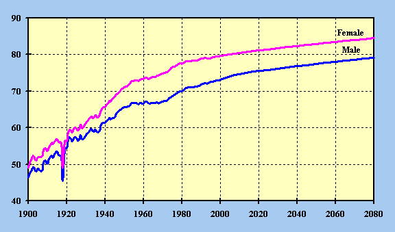
Table 9 gives the resulting life expectancies at birth and age 65 for males and females respectively, for historical years and by alternative for selected future years. Life expectancy for any year is the number of years of life remaining for a person who is assumed to experience the death rates by age observed in or assumed for the selected year. Thus, the life expectancies at birth and at age 65 shown in Table 9 are summary statistics of the overall mortality for the applicable calendar year.
Rapid gains in life expectancy at birth occurred from 1900 through the mid-1950's for both males and females. From the mid-1950's through the late 1960's, male life expectancy at birth remained level, while female life expectancy at birth increased moderately. During the 1970's rapid gains resulted for both males and females. Through the 1980's until the present, life expectancy at birth has been increasing less rapidly. During this century life expectancy at birth for males increased 25.8 years from 46.4 in 1900 to 72.2 years in 1994. During the same period, life expectancy at birth for females increased 30.0 years from 49.0 to 79.0 years. Thus the difference in male and female life expectancies, the sex gap, at birth has increased from 2.6 years in 1900 to 6.8 years in 1994. The sex gap in life expectancy at birth reached peaked in calendar year 1970, at 7.7 years. The sex gap stabilized during the 1970's and has decreased slightly since 1979. Figure 2 is a graph of the past and projected life expectancies at birth of males and females from 1900 to 2080, for historical years and projected for the intermediate assumption.
|
Figure 2. - Male and Female Life Expectancy
(in years) 1900-2080 Actual and Projected Intermediate Alternative |
|
| Calendar Year |
Under all three alternatives, the life expectancy at birth is projected to increase. For males, the life expectancy at birth increases from 72.2 years in 1994 to 76.2 years, 79.2 years, and 83.4 years in 2080 under the low cost, intermediate and high cost alternatives, respectively. This represents an increase ranging from 4.0 years to 11.2 years. For females the increase ranges from 2.3 years to 9.8 years. The female life expectancy is projected to increase from 79.0 years in 1994, to 81.3 years, 84.5 years, and 88.8 years in 2080 under the low cost, intermediate and high cost alternatives, respectively. The sex gap at birth is projected to decrease from 6.8 years in 1994 to 5.2 years in 2080 under the low cost alternative, to 5.3 years under the intermediate alternative, and 5.4 years under the high cost alternative.
Life expectancy at age 65 for males increased from 11.3 years in 1900 to 15.3 years in 1994, while life
expectancy at age 65 for females increased from 12.0 years to 19.0 years. The life expectancy for males
at age 65 is projected to increase from 15.3 years in 1994 to 16.6 years, 19.0 years, and 22.3 years in
2080 under the low cost, intermediate and high cost alternatives, respectively. This represents an increase
ranging from 1.3 years to 7.0 years. For females the increase from 1994 through 2080 ranges from 0.8
years to 7.0 years. The female age 65 life expectancy is projected to increase from 19.0 years in 1994
to 19.8 years, 22.5 years, and 26.0 years in 2080 under the low cost, intermediate, and high cost
alternatives, respectively. The sex gap in life expectancy at age 65 increased from .7 years in 1900 to
4.4 years in 1979. Since then, this gap has decreased slightly to 3.7 years in 1994 and, in 2080, is
projected to be 3.2 under the low cost alternative, 3.5 under the intermediate alternative, and 3.7 under
the high cost alternative.
3. Net Immigration
Immigration was once a very important element in the growth of the United States population. For each year 1870 through 1930, the population averaged about 13 percent foreign born. Figures published by the Bureau of the Census in Current Population Reports in The Foreign-Born Population: 1996, No. PC20-494, March 1997, indicate the percentage of foreign born declined to a low of about 5 percent in the 1970 Census, rose to about 8 percent in the 1990 Census and is currently estimated to be just over 9 percent.
Legal immigration averaged nearly one million per year from 1904 through 1914. Immigration decreased greatly during World War I and following the adoption of quotas based on national origin in 1921. The economic depression in the 1930's caused an additional but temporary decrease which resulted in more emigration than immigration. Annual legal immigration increased after World War II to around 300,000 persons per year and stayed at that level through the 1950's and into the 1960's.
With the Immigration Act of 1965 and other related changes, annual legal immigration increased to about 400,000 and remained fairly stable until 1977. For the years 1977 through 1991, legal immigration (excluding aliens admitted under the Immigration Reform and Control Act of 1986) averaged approximately 580,000 per year. This increase was due to the increase in numbers of relatives admitted and to the large numbers of refugees and political asylees that were admitted based on specific legislation during this period.
The Immigration Reform and Control Act of 1986 (IRCA) permitted aliens who could provide evidence that they had been residing in the United States illegally since 1982, or since 1986 for certain agricultural workers, to apply directly for permanent residency. 2.7 million persons were legalized during 1989 through 1993 under this legislation. These new immigrants had previously been included in the population as other-than-legal aliens.
For the years 1989 through 1991, a previously unused provision of the Immigration Act of 1965 was implemented to issue visas over and above the 270,000 numerical limit to persons in countries adversely impacted and/or under represented by the Immigration Act of 1965. Most of the additional visas have gone to natives of Ireland, Canada, Poland, and Indonesia. In 1989, 15,000 such visas were issued with an additional 25,000 in 1990 and 40,000 in 1991.
The historical numbers of immigrants in tables 10 and 11 are from the 1995 Statistical Yearbook of the Immigration and Naturalization Service.
The Immigration Act of 1990, which took effect in fiscal year 1992, restructured the immigration categories and substantially increased the number of immigrants who may legally enter the United States each year. The 1990 law did away with the old numerically limited and immediate-relative categories and replaces them with family-sponsored preference, employment-based preference, and diversity categories for immigration. A cap of 675,000 immigrants per year was set for 1995 and later. This cap is referred to as "pierceable" because unused visas from prior years and other specially legislated immigrants are not included in these ceilings. The maximum number of refugees, which is set annually, was 112,000 for 1995. The following table gives the maximums for both the 1965 Act and the 1990 Act, using the categories created under the 1990 Act.
| Legal Immigration Limits | |||||
| | | | 1965 Act | 1990 Act | |
| 1992-1994 | 1995 and later | ||||
| Flexible Cap | 500,000 | 700,000 | 675,000 | ||
| Family Preference | 440,000 | 520,000 | 480,000 | ||
| Immediate Relatives | 225,000 | 239,000 | 254,000 | ||
| Family Sponsored | 215,000 | 226,000 | 226,000 | ||
| IRCA Families | -- | 55,000 | -- | ||
| Employment Based | 60,000 | 140,000 | 140,000 | ||
| Diversity Immigrants | -- | 40,000 | 55,000 | ||
| Separately Set Limits | |||||
| Refugees* | 95,000 | 130,000 | 120,000 | ||
| Asylees | 5,000 | 10,000 | 10,000 | ||
| * Refugee numbers are set annually. The numbers shown here are averages of available data years. | |||||
The historical numbers of immigrants, by the 1990 Act's categories, are shown in table 11.
Other factors affecting the level of legal immigration include but are not limited to: application processing backlogs, shifting of responsibilities from Department of State to the Immigration and Naturalization Service (INS), economic changes in the United Sates and abroad and anti-immigrant sentiment in the US. These factors are having a greater impact than expected on the numbers of immigrants, causing the numbers to be lower than expected for fiscal year 1995. The lower immigrant numbers are expected to be temporary. The projection of legal immigrants for Alternative II, therefore, drops below 800,000 for years 1995 through 1999, rising to an ultimate rate of 800,000 per year for years 2000 and later.
Statistics on emigration are sparse and largely estimated (see, "Foreign-Born Emigration From the United States: 1960 to 1970" by Robert Warren and Jennifer Peck in Demography, February 1980). However, research done by the Immigration and Naturalization Service and other experts estimates emigration to be in the range of 20-40 percent of legal immigration. Emigration from the Social Security Area is expected to be less than emigration from the United States, especially at the older ages, primarily because individuals who leave the United States having achieved fully insured status are still eligible to receive OASDI benefits and thus are still considered to be in the Social Security Area. In the 1996 Trustees Report, an emigration/immigration ratio of 25 percent was used for all three alternatives. For the 1997 Trustees Report we are varying our emigration ratio to assume 20, 25 and 30 percent for the low cost, intermediate and high cost alternatives, respectively.
In determining the ultimate level of net legal immigration for the intermediate alternative, the following assumptions are made:
(1) 675,000 immigrants admitted per year under the family-based, employment-based and diversity categories, the flexible cap in the 1990 Immigration Act
(2) 125,000 asylees, refugees and other miscellaneous immigrants, levels for these categories set annually by the President and the Congress
(3) Emigration is estimated to be approximately 25 percent of the level of legal immigration
This results in an intermediate assumption of 600,000 per year for the intermediate alternative net legal immigration for years after 2000. The ultimate levels of net legal immigration for years after 2000, for the low and high cost alternatives are assumed to be 700,000, and 550,000 persons per year, respectively.
The age-sex distribution of the assumed legal immigration was based on data supplied by the INS on immigration during 1978 through 1995. The age-sex distribution of the assumed legal emigration was based on estimates of foreign-born emigration for 1960 to 1970 in "Foreign-Born Emigration From the United States: 1960 to 1970" by Robert Warren and Jennifer Peck in Demography, February 1980. Table 12 shows the age-sex distributions of the annual net legal immigration (excess of immigration over emigration) assumed for the ultimate, years 2000 and later.
In deciding upon the level of annual net immigration to be assumed for future years, the possibility of making some provision for persons not legally entering the United States arises. Estimates of these aliens are included in our starting population, in accordance with the official policy of the Bureau of Census to enumerate or to include in the estimated undercount all persons residing in the U.S. In a recent joint project, INS and the Bureau of Census examined the illegal immigrant population between October 1988 and October 1992. Not counting those who would be subsequently legalized under the IRCA program, there were still estimated to be 2.2 million illegal immigrants in the population as of October 1988. At the time of the 1990 census there were estimated to be 2.6 million illegals, increasing by October 1992 to 3.4 million. The INS is currently in the process of revising its estimates of net illegal immigration based on information provided by persons legalized under IRCA, counts of unauthorized immigrants in Census surveys, and the number of overstays of legally admitted persons. INS estimates that between 1988 and 1992, illegal immigration averaged 300,000 persons per year, numbers significantly higher than the 200,000 estimate based on 1980 Census data.
Even after considering the effects of recent legislation, annual net other-than-legal immigration is
anticipated to continue, because of the limited economic opportunity in the native countries of the
majority of these aliens. Because of this expectation, for years after 1995 the intermediate alternative
assumption for annual net other-than-legal immigration is 300,000. For the low and high cost
alternatives, the corresponding numbers are 450,000 and 200,000, respectively. The age-sex distribution
of the other-than-legal immigrants was based on unpublished Bureau of Census estimates of the
undocumented population counted in the 1980 Census. Table 13 shows the age-sex distribution of the
assumed net other-than-legal immigration for the three Alternatives.
4. Marriage
Because marriage is the combination of a male and a female into a couple, marriage rates can be computed as a ratio of the number of marriages to the number of nonmarried males (not taking into account the number of nonmarried females), the number of nonmarried females (not taking into account the number of nonmarried males), or a theoretical number of nonmarried couples that takes into account both the number of nonmarried males and nonmarried females. The marriage rates referred to in this study are computed using the third concept of a theoretical number of nonmarried couples as the denominator. The rates were computed as the number of marriages for given ages of husband and wife divided by the square root of the product (geometric mean) of the midyear nonmarried males and nonmarried females of the given ages.
In order to calculate these rates, data on new marriages in the Marriage Registration Area (MRA) were obtained from the National Center for Health Statistics for calendar years 1957 through 1988 by age of husband crossed with age of wife. In 1988, the MRA consisted of 42 States and D.C. and accounted for 80 percent of all marriages in the U.S. Estimates of the nonmarried population in the MRA were obtained from NCHS by age and sex.
The number of marriages depends upon the age distribution of both the nonmarried male population and the nonmarried female population. Thus, an acceptable summary statistic for the marriage rate could be calculated by age-adjustment to a set of standard nonmarried populations. When only one population is involved (as in calculating death rates), equal results are obtained by viewing the age-adjusting concept as the weighted average of the age-specific rates or as the crude rate that would occur in the standard population. When two populations are involved (as in calculating marriage rates), these two concepts do not produce the same results.
Using either concept, the first step in calculating the age-adjusted marriage rate is to determine the number of marriages that would occur in the standard population. This number, the expected number of marriages, is determined by applying the age-of-husband-age-of-wife-specific marriage rates to the geometric mean of the corresponding standard age-specific populations. To age-adjust using the weighted average concept, the expected number of marriages is divided by the sum of all of the factors to which the marriage rates were applied, i.e., the sum of the geometric means of the corresponding age-specific populations. To age-adjust using the crude rate concept, the expected number of marriages is divided by the geometric mean of the total male nonmarried population and the total female nonmarried population. In this study we have calculated rates (as shown in figure 3 and table 14) under the latter concept, i.e., the crude rate that would be experienced in the standard population, which we express per hundred thousand nonmarried of each sex.
The first step in calculating the total age-adjusted central marriage rate for a particular year is to determine an expected number of marriages by applying the age-of-husband age-of-wife specific central marriage rates for that year to the square root of the product of the corresponding age groups of unmarried males and unmarried females in the MRA as of July 1, 1982. The total age-adjusted central marriage rate is then obtained by dividing the expected number of marriages by the square root of the product of the number of unmarried males, ages 15 and older, and the unmarried females, ages 15 and older in the MRA as of July 1, 1982. The rates in table 14 were obtained by this method.
An examination of the age-adjusted marriage rates since 1957 shows that the rates remained relatively stable during the late 1950's and throughout the 1960's. A major decrease in the age-adjusted rate was experienced during the 1970's and continued into the 1980's. The total rates shown in table 14 and in figure 3 range from a high in 1968 of 10,168 per hundred thousand nonmarried persons of each sex to a low in 1988 of 5,032. At first glance the statistics for 1989 through 1995, as shown in table 14, indicate a rise in the marriage rate. The provisional age-adjusted marriage rates are based on United States data, which historically produce higher rates than the MRA data. This is because the MRA does not include the state of Nevada, a state which marries large numbers of out-of state residents. In order to compare the rates determined from the two sources of data, a factor in the neighborhood of .9 should be applied to the age-adjusted marriage rates based on U.S. data. Once this factor is applied, the provisional age-adjusted marriage rates for 1989 through 1995 indicate a continuation, yet slowing down, of the declining trend.
Because of uncertainty whether marriage rates will increase or decrease, we assumed for the intermediate alternative that future age-adjusted rates of marriage for the Social Security Area would continue to slowly decrease and then stabilize in 2021. The age-adjusted marriage rate in 2021 is assumed to equal approximately 95 percent of the average of the age-adjusted marriage rates for the period 1989 through 1995. The use of constant age-adjusted rates does not imply that the crude rate of marriage in the projected population remains constant.
While it is possible that marriage rates will continue to decline, it is not likely that the rate of decline of recent history will continue indefinitely into the future. Taking this into account, for the low cost alternative, we assume that the ultimate age-adjusted marriage rate will decline to 4,000 in the year 2021 and stay at this level for the remainder of the projection period. It is also possible that marriage rates will, on the average, rise above their present low level. We, however, believe that the rates will not, on the average, return to the high levels found in the 1950's and 1960's. To reflect this in the high cost alternative, we assume that the ultimate age-adjusted marriage rate will increase to 9,000 in the year 2021 and stay at this level for the remainder of the projection period.
|
Figure 3. - Age-Adjusted Marriage Rates
(per hundred thousand unmarried of each sex) in the MRA, 1957-1995 |
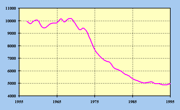 |
| Calendar Year |
To obtain the age-of-husband-age-of-wife-specific rates for a particular year from the age-adjusted rate projected for that year, the age-of-husband-age-of-wife-specific rates for the years 1978 and 1979 and 1981 through 1988 were averaged, graduated, and proportionally ratioed so as to produce the age-adjusted rate for the particular year. Data for 1980 were not available. The rates assumed for years after 1995 for the intermediate alternative are shown in table 15 grouped by 5 year age groups based on Social Security Area population as of July 1, 1995.
A complete projection of age-of-husband-age-of-wife-specific marriage rates was not done separately for
each previous marital status. However, experience data indicate that the differential in marriage rates by
previous marital status is significant. Future relative differences in marriage rates by previous marital
status were assumed to be the same as the average of those experienced during 1979 and 1981 through
1988. Data for 1980 were not available. The marriage rates for the years 1979 and 1981 through 1988
were obtained from unpublished data supplied by the National Center for Health Statistics. The average
of these marriage rates, with slight modifications, grouped by 5-year age groups based on the MRA
population as of July 1, 1982, are given in table 16.
5. Divorce
Data on divorces (including annulments) in the Divorce Registration Area (DRA) during calendar years 1979 through 1988 by age group of husband crossed with age group of wife, were obtained from the National Center for Health Statistics. For each of the above calendar years, the number of divorces occurring in the DRA (which in 1988 consisted of 31 States and accounted for about 48 percent of all divorces in the U.S.) were inflated to represent the Social Security Area, based on the total number of divorces during the corresponding calendar year in the 50 States, the District of Columbia, Puerto Rico, and the Virgin Islands. Divorce rates for each age of husband crossed with each age of wife were then calculated as the ratio of the inflated number of divorces in the Social Security Area for the given age of husband and age of wife to the number of existing marriages in the Social Security Area with the given age of husband and age of wife. Table 17 contains the resulting rates, age-adjusted to the married Social Security Area population as of July 1, 1982.
As shown in table 17, the age-adjusted central divorce rates were quite stable during the period 1979 through 1988. Age-adjusted central divorce rates for 1989 through 1995 were computed using the age distributions of the DRA data during 1979 through 1988 and using provisional data estimating the total divorces in the U.S. for 1989 through 1995. The resulting age-adjusted rates are slightly lower than those for 1979 through 1988. For 1996, the age-adjusted central divorce rate was assumed to be equal to the average of the age-adjusted rates for the seven provisional years for all three alternatives.
Because age-adjusted central divorce rates have remained fairly constant over the last ten years, we assumed under the intermediate alternative that throughout the projection period the age-adjusted rate would remain close to the same level as that recently experienced. For the low cost alternative, we assumed that the age-adjusted rate would gradually increase to approximately 110 percent of the 1995 estimated value in 25 years and then remain at this level throughout the remaining projection period. For the high cost alternative, age-adjusted rates are assumed to decrease, reaching approximately 85 percent of the 1995 estimated rate in 25 years and then to remain constant throughout the remaining projection period.
To obtain age-specific rates for use in the projections, the age-of-husband-age-of-wife-specific rates for
the years 1979 through 1988 were averaged and then graduated. For each alternative and year after
1995, the averaged and graduated rates were adjusted by a factor so as to produce the age-adjusted
central divorce rate assumed for that particular year and alternative. The rates assumed for years after
1995 for the intermediate alternative are shown in table 18 grouped by 5 year age groups based on
Social Security Area population as of January 1, 1990.
D. Methods
Future numbers of births, deaths, net immigrants, marriages, and divorces are estimated by applying the following methods to the projected data described in the preceding section. End of year population data is determined from the beginning of year population data.
Estimates of the size of the single (never married) population at the end of the year, for each age and
sex, are calculated from the estimated single population at the beginning of the year by subtracting the
number of deaths and marriages among single persons during the year, and adding the number of net
immigrants of single persons during the year. The married population at the end of the year is calculated
from that at the beginning of the year by subtracting estimates of the numbers of deaths, widowings, and
divorces during the year, and adding estimates of the numbers of marriages and net married immigration
during the year. Similarly, the widowed population at the end of the year is calculated by subtracting
the deaths and marriages, and adding the widowings and the net immigration of widowed persons. The
divorced population at the end of the year is calculated by subtracting the deaths and marriages, and
adding the divorces and the net immigration of divorced persons.
1. Fertility
In order to determine the number of births during a year, birth rates for that year were applied to the
average of the beginning-of-year and end-of-year female population. Projected numbers of births are
given in table 20 by alternative.
2. Mortality a. Probability of Survival
Earlier in this study, death rates (generally referred to as central death rates) were presented which were calculated as the number of deaths occurring in a given year divided by the midyear population in that year. This concept is a useful one in the context of analyzing historical trends, but is not so readily applicable to the actual projection of population. What is more suitable is the concept of probability of death (or of survival). This concept involves dividing the number of deaths occurring to a group in a given year by the number of persons in that group at the beginning of the year (rather than the population at the middle of the year). As one would expect, these two concepts are closely related, although the mathematics of their relationship is not trivial.
Future probabilities of survival by age last birthday were calculated for each sex and each single year of age from the projected central death rates by sex and age group. For each future year in the projection period, the probability of death at age 0 was calculated from the projected central death rate for age 0 assuming that the relationship between the probability of death and the central death rate that existed in 1994 remained constant. For each single year of age 1 through 4, probabilities of death were calculated in the same manner using central death rates for the age group 1 through 4 (4m1). Probabilities of death at ages 5 and older were calculated by an iterative method. As a first approximation, the probability of death for each five year age group from 5 through 9 to 90 through 94 was calculated from the corresponding central death rate assuming that on the average deaths occurred at the middle of the age interval. As part of the iterative process, the probability of death for each single age in each five-year age group was determined by interpolating the logarithms of the complements of the surrounding five-year probabilities of death with Beer's minimized fifth-difference formula. The probability of death for each age 95 and over was calculated to produce a rapid decline in the ratio of succeeding probabilities of death to a minimum ratio of 1.06 for females and 1.05 for males. These ratios were chosen based on the analysis by Francisco R. Bayo and Joseph F. Faber contained in the paper "Mortality Experience Around Age 100," in the Transactions of the Society of Actuaries, Volume XXXV.
An initial life table for each sex was then constructed using these probabilities of death. On subsequent iterations, the life table probability of death for each age 5 through 94 was adjusted so that the central death rates for the five-year age groups obtained by weighting the single age life table central death rates by the population would equal the corresponding population five-year age group central death rates. This adjustment corrects for the fact that the distribution within each quinquennial age group in the life table population generally differs from that in the actual population. For more detail on the method used to produce the life tables for these population projections see Actuarial Study No. 107, "Life Tables For The United States Social Security Area: 1900-2080" by Felicitie C. Bell, Alice H. Wade and Stephen C. Goss.
Table 19 is the life table for 1994, the last calendar year that complete data was available. The standard actuarial functions presented in table 19 are defined below.
| = | the probability that a person exact age x will die within one year | |
| = | the number of persons surviving to exact age x, or the number of persons reaching exact age x during each year in the stationary population | |
| = | the number of person-years lived between exact ages x and x+1, or the number of persons alive at age last birthday x at any time in the stationary population | |
| = | the number of person-years lived after exact age x, or the number of persons alive at age last birthday x or older at any time in the stationary population | |
| = | the average number of years of life remaining at exact age x |
The number of deaths occurring at each age and sex was calculated as the difference between the number of people alive at the beginning of the year and the product of the number of people alive at the beginning of the year and the probability of survival. Deaths to newborn babies were computed using a similar formula. However, deaths to immigrants newly arriving in the year were disregarded. The numbers of deaths were then distributed by marital status in the same proportions as would have been produced by applying the marital-status specific probabilities of survival to the population by marital status at the beginning of the year. Projected numbers of deaths are given in table 20 by alternative.
The number of marriages dissolved by death at each age of husband crossed with each age of wife was calculated by applying joint-life probabilities of death to the existing marriages by age of husband crossed with age of wife at the beginning of the year. (The joint-life probabilities were developed to be consistent with the projected death rates and the assumed mortality differential by marital status, and assumed independence of the partners). The number of widowings for a particular age and sex was calculated as the difference between the marriages of individuals of that particular age and sex dissolved by death of either partner and the number of deaths to married persons of that age and sex.
The assumed net immigration for each age and sex was distributed among the single (never married), married, widowed, and divorced populations based on the proportions as existed in the nonmarried (single plus widowed plus divorced) population at the beginning of the year. Adjustments were required in order to ensure that the numbers of net married immigrants would be consistent with the estimates of the married population by age of husband crossed with age of wife at the beginning of the year.
The number of marriages occurring at each age of husband crossed with each age of wife is, in theory, obtained by multiplying the age-of-husband-age-of-wife-specific marriage rates with the geometric mean of the midyear male population exposed to marriage and the midyear female population exposed to marriage. Thus, the midyear populations exposed to marriage must be estimated from the beginning of the year nonmarried populations. Because the midyear populations exposed to marriage depend on the number of marriages during the first half of the year, the process of obtaining the number of marriages is performed iteratively.
As a first approximation, the midyear male population exposed to marriage was calculated by age as the average of the number of nonmarried males at the beginning of the year and an estimate of the number of nonmarried males at the end of the year. The nonmarried male population at the end of the year was estimated from the population at the beginning of the year by subtracting deaths and adding new immigrants, widows, and divorces during the year. The female population exposed to marriage was approximated similarly. As a second approximation, the midyear male population exposed to marriage was calculated in the same manner as the previously calculated midyear male population of the given age exposed to marriage less one-half of all marriages involving men of the given age. (The number of marriages being obtained by using the first midyear nonmarried population approximations). The female population exposed to marriage was similarly approximated. The difference between the number of marriages obtained by using the two midyear population approximations was calculated. The iterative process was continued until the difference between the number of marriages was small. The numbers of marriages were then distributed by previous marital status in the same proportions as would have been produced by applying the previous marital-status-specific marriage rates to the population by marital status at the beginning of the year. Projected numbers of marriages are given in table 20 by alternative.
The number of divorces during a year occurring at each age of husband crossed with each age of wife is, in theory, obtained by multiplying the age-of-husband-age-of-wife-specific divorce rates for that year with the midyear number of married couples in that age crossing. Because the numbers of marriages by age of husband crossed with age of wife are only available as of the beginning of the year, midyear estimates of these numbers must be made. In addition, because these estimates depend on the number of marriages and divorces occurring during the first half of the year, the process of obtaining these estimates is performed by a series of iterations.
For the first iteration, the numbers of new marriages during the first half of the year is assumed to be zero. As a first approximation, for each age of husband crossed with age of wife, the midyear married population is estimated from the beginning of year married population by adjusting for the number of widowings, dissolutions occurring when both husband and wife die, and net immigrants during the first half of the year. As second approximation, the married population is calculated in the same manner with an additional adjustment of subtracting one-half of all divorces occurring during the year to couples of those age crossing. (The number of divorces being obtained by using the first midyear married population approximations). The total numbers of divorces over all age crossings using the two midyear married population approximations were calculated and the totals was determined. The first iterative process was continued until the difference between the successive totals was small.
For the second iteration, the process above was repeated except using an additional adjustment of adding in one-half of the new marriages to all of the midyear population calculations. (The number of new marriages being estimated by an iterative process as described in the next section). This process was continued until the iteration series described above and the iteration described in the next section, using the most recent estimates of numbers of new divorces, were completed with acceptable results. Projected numbers of divorces are given in table 20 by alternative.
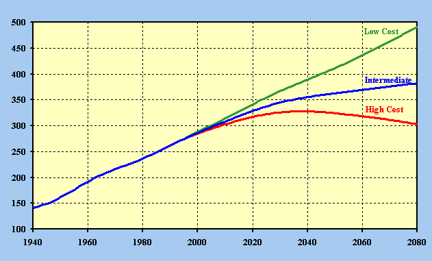
III. Results A. Total Population
Table 21 displays the resulting Social Security Area population by age group, sex, marital status, and alternative as of January 1 for selected historical (table 21a) years. The past and projected total population is shown graphically in figure 4. Under the low cost (table 21b) alternative (with greater-than-replacement fertility), the total population increases rapidly from 272 million in 1995 to 488 million in 2080. Under the intermediate (table 21c) alternative, the total population increases gradually to 381 million in 2080. Under the high cost (table 21d) alternative, the total population increases to 328 million in 2040 and then decreases to 304 million in 2080, due to the compounding effect of below-replacement fertility which is only partially offset by the positive net immigration.
|
Figure 4. - Social Security Area Population
(in millions), 1940-2080 Actual and Projected by Alternative |
|
| Calendar Year |
Table 22 and figure 5 illustrate the change in the median age of the total population and over 65 population throughout the projection period. The median age of the total population has been increasing since 1970. For the intermediate alternative, the median age is projected to increase slowly over the entire projection period. The mean age of the population 65 and older has increased approximately six years since 1940. For the intermediate alternative, the median age of the 65 and older population is projected to increase slightly until the year 2006, decline slightly during the next 15 years, resume increasing until 2043, and then to fluctuate mildly for the remainder of the period.
The patterns of increase are mainly due to past and assumed future patterns of fertility. The aging and dying off of the "baby boom generation" (those born during the late 1940's through the mid 1960's) is a major reason for the median age of the population 65 and older increasing slightly, then stabilizing. Also contributing to the increase in median age is the assumed decrease in mortality. As people are assumed to live longer, the median age of the population increases. This factor has more effect on the median age under the high cost alternative, where greater mortality reductions are assumed. Sustained higher future fertility rates, as assumed for the low cost alternative tend to keep the median age at lower levels.
|
Figure 5. - Median Age of Total Population and 65 and over Population
Actual and Projected Intermediate Alternative |
|
| Calendar Year |
B. Population by Marital Status
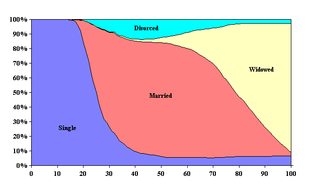
Marital status is important in determining benefit costs, present and future. In 1995, 42 percent of the population was estimated to be single (never married), 46 percent currently married, 6 percent widowed and 6 percent divorced.
Figures 6a and 6b show the distribution of the population by marital status in 1995, and the projected distribution under the intermediate alternative in 2080, respectively.
|
Figure 6a. - Distribution of the Population by Marital Status,
Ages 0 through 100 January 1, 1995 |
|
| Calendar Year |
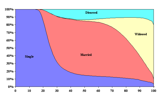
The proportion of the population which is projected to be single in 2080 under the intermediate alternative is 39 percent, 3 percentage points less than current levels, reflecting differences in the age distribution of the population. Particularly interesting to note is the increase in never marrieds over age 40, from less than 10 percent in 1995 to greater than 10 percent in 2080. The proportion projected to be married under the intermediate alternative is 46 percent, the same as current levels. The proportion
widowed in 2080 is also projected to be unchanged, at 6 percent. The current high incidence of divorce and the future assumptions concerning marriage and divorce result in an increase in the proportion divorced to 8 percent by 2080. The percent divorced among the 60 and older is at or above the 10 percent level, much different from the less than 10 percent of today.
|
Figure 6b. - Distribution of the Population by Marital Status,
Ages 0 through 100 January 1, 2080 Intermediate Alternative |
|
| Calendar Year |
The proportion of the population in 2080 under the low cost alternative which is projected to be single is 49 percent, married is 37 percent, widowed is 5 percent and divorced is 9 percent. The proportion of the population in 2080 under the high cost alternative which is projected to be single is 25 percent, married is 59 percent, widowed is 8 percent and divorced is 7 percent. The spread among the alternatives reflects the differences in the projected marriage and divorce rates and in the age distribution of the population among the three alternatives.
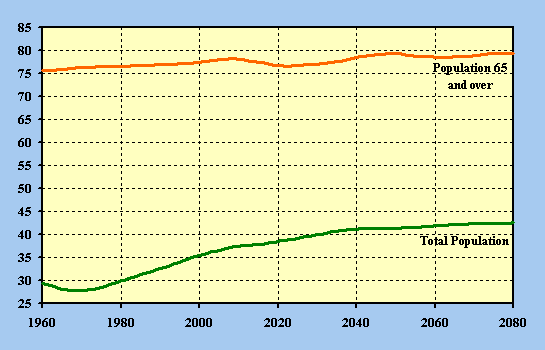
A rough estimate of the growth in the number of persons receiving Social Security retirement benefits can be obtained from examining the population age 65 and older given in table 23. The projected population at age 65 and older is also shown graphically in figure 7. The growth in the number of people age 65 or older slows down around the year 2000 due to the low fertility experience during the 1930's. This slowing down is not as great under the intermediate and high cost alternatives because assumed mortality reductions are greater than under the low cost alternative. The high fertility of the 1950's and 1960's results in sharp steady growth in the population age 65 and older for the period 2010 through 2030 under all of the alternatives. By the year 2080, the population age 65 and older has increased significantly as a percentage of total population from 13 percent in 1995, to 17 percent under the low cost alternative, 23 percent under the intermediate alternative, and 31 percent under the high cost alternative.
|
Figure 7. - Social Security Area Population Aged 65 and Older
(in millions), 1940-2080 Actual and Projected by Alternative |
|
| Calendar Year |
Table 22 and figure 5 show the change in the median age of the population ages 65 and older. This median age increases until around 2010, when the "baby boom generation" begins to reach 65. As the "baby boom generation" ages, the median age once again increases. At the same time the "baby boom generation" ages, the low fertility period of the 1970's and early 1980's also contributes to the increase in the median age. In addition to the historical fertility experience, mortality reduction is also a factor in the change in the median age of the population ages 65 and older. In general, with all other factors held constant, reductions in mortality result in longer life and higher median age.
The projected population is summarized in table 23 by broad age group, marital status and alternative for selected years. The age groups are under 20 years, 20-64 years, and 65 years or older. Marital status categories are single (never married), currently married, currently widowed, and currently divorced. No information about prior marital status is included. Therefore, the marital status shown is the status the person is currently in, as of the year shown.
The disunity ratio given in table 23 is the ratio of the number of divorced persons to the sum of the numbers of married and widowed persons. This ratio is assumed to increase from .122 in 1995 to .212 and .160 in 2080 under the low cost and intermediate alternatives, respectively, and to decrease to .101 in 2080 under the high cost alternative.
The total dependency ratio given in table 23 is the ratio of the number of persons who are under age 20 or over age 64 to the number of persons aged 20 through 64. This ratio views the possible future financial burdens to be borne by workers from a somewhat broader perspective. Under all three alternatives, the total dependency ratio is projected to decrease from .709 in 1995 to a minimum around 2010, reflecting the small number of children resulting from the low fertility rates experienced since 1970 and projected to be experienced in the near future, and the slow growth in the aged population resulting from the low fertility rates experienced during the 1930's. Shortly after 2010, the total dependency ratios begin to rise, largely reflecting the same effects that influence the aged dependency ratios. Projected values of the total dependency ratio in 2080 range from .802 under the low cost alternative to .945 under the high cost alternative or roughly from 13 to 33 percent higher than the 1995 value.
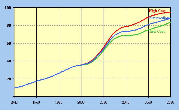
The aged dependency ratio shown in table 23 and figure 8 is the ratio of the number of persons aged 65 or older to the number of persons aged 20 to 64. This ratio is closely related to the ratio of retirees to workers and, thus, provides an index of possible future demographic pressures which may be faced by the OASDI program. The Social Security Amendments of 1983, in order to insure the continued ability of Social Security to pay benefits, raised the normal retirement age. For workers who attain age 62 in 2000 through 2004, eligibility age for full benefits (called the normal retirement age) is increased to age 65 plus two months for each year after 1999 the worker attains age 62. This raises the normal retirement age to 66 in 2005 for persons born in 1943 through 1954. The normal retirement age is again raised for workers who attain age 62 in 2017 through 2021 to age 66 plus two months for each year after 2016 the worker attains age 62. This raises the normal retirement age to 67 for persons born in 1960 and later. Information provided in table 21a (historical), table 21b (low cost alternative), table 21c (intermediate alternative), and table 21d (high cost alternative), allows calculation of the aged dependency ratios for retirement ages 65 through 70.
Under the low cost alternative, the aged dependency ratio for retirement age 65 is projected to increase from 0.214 in 1995 to 0.327 in the year 2035 and then to decrease to an ultimate level of 0.308. Under the intermediate alternative, the aged dependency ratio for retirement age 65 is projected to decrease slightly until 2005, then to steadily increase to 0.421 in 2080. Under the high cost alternative, the aged dependency ratio for retirement age 65 is projected to decrease slightly until 2005, then to steadily increase to 0.608 in 2080. A sharp increase in the aged dependency ratio shortly after the turn of the century appears certain as the "baby boom generation" attains age 65 while the "baby bust" generation'' (those born during the 1970's and 1980's) attains age 20. The magnitude of the increase, however, will depend upon future mortality reductions among the aged and future fertility rates. Even under low cost assumptions, however, the aged dependency ratio will have increased about 50 percent by the year 2030.
|
Figure 8. - Aged Dependency Ratio, 1940 through 2080
(Ratio of Population Aged 65 and older to Population Aged 20 through 64) Actual and Projected by Alternative |
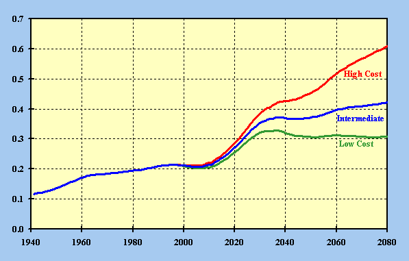
|
| Calendar Year |
Since not everyone retires at age 65 and since the minimum age at which unreduced benefits are payable is scheduled to increase, it is interesting to observe the aged dependency ratio using cutoff ages other than 65. Table 24 displays these ratios at age 62, when retired worker benefits are first available; at age 65, the current normal retirement age; at age 66, which will be the normal retirement age beginning in 2005; at age 67, which will be the normal retirement age beginning in 2022; at age 70, after which delayed retirement credits can no longer be earned; and at ages 72 and 75. The normal retirement age is the minimum age at which unreduced retirement benefits are payable. People at ages lower than the normal retirement age receive reduced benefits.
In table 25 the normal retirement ages necessary to maintain aged dependency ratios of .20, .25, and .30 are given. In order to maintain an aged dependency ratio of .20, the approximate age 65 dependency ratio during the period 1980 through 1990, the aged dependency ratio in 2080 must be calculated at ages 71, 75, and 80 under the low cost, intermediate and high cost alternatives, respectively. Under all three alternatives, the normal retirement age necessary to maintain a selected aged dependency ratio increases rapidly from 2010 to 2040.