A Progressivity Index for Social Security
Issue Paper No. 2009-01 (released January 2009)
Using the Social Security Administration's MINT (Modeling Income in the Near Term) model, this paper analyzes the progressivity of the Old-Age, Survivors and Disability Insurance (OASDI) program for current and future retirees. It uses a progressivity index that provides a summary measure of the distribution of taxes and benefits on a lifetime basis. Results indicate that OASDI lies roughly halfway between a flat replacement rate and a flat dollar benefit for current retirees. Projections suggest that progressivity will remain relatively similar for future retirees. In addition, the paper estimates the effects of several policy changes on progressivity for future retirees.
Andrew Biggs, currently a Resident Scholar at the American Enterprise Institute, was with the Social Security Administration when this paper was written. Mark Sarney and Christopher R. Tamborini are with the Office of Retirement Policy, Office of Retirement and Disability Policy, Social Security Administration. Questions about the analysis should be directed to them at 202-358-6295 or 202-358-6109 respectively.
Acknowledgments: The authors wish to thank Lakshmi K. Raut, Lee Cohen, Dean Leimer, Dave Shoffner, David Pattison, and David Weaver for their insightful comments and suggestions on earlier drafts. The authors also benefited from the comments of the editors.
The findings and conclusions presented in this paper are those of the authors and do not necessarily represent the views of the Social Security Administration.
Summary and Introduction
The Social Security benefit formula has incorporated some measure of progressivity almost since the program's inception. As early as 1939, amendments to the original Social Security Act stipulated that monthly benefits replace a higher proportion of preretirement earnings for people with lower earnings compared with those with higher earnings (Martin and Weaver 2005). Throughout the program's history, benefit adequacy—promoted through a progressive benefit formula—has been balanced with equity, the goal that benefits increase with contributions.
Although the Social Security retirement system is designed to replace a higher percentage of earnings for lower-income workers and their dependents,1 the degree to which the program actually achieves progressive outcomes is less certain. To contribute to our understanding of this issue, this paper introduces a new measure—a progressivity index—to estimate the progressivity of the Social Security retirement program. Our purpose is to develop a comprehensive, easy-to-understand summary measure for evaluating the magnitude of progressivity under Social Security within cohorts and for assessing potential shifts in systemwide progressivity as a result of policy changes.
Social Security progressivity can be described in various ways. For the purposes of this paper, we define progressivity as the degree to which benefits are higher relative to lifetime payroll contributions for lower contributors than for higher contributors. This definition can be related to Musgrave and Thin's note (1948) regarding the income tax:
It is generally agreed that a rate structure is progressive where the average rate of tax (i.e., tax liability as a percentage of income) rises when moving up the income scale; proportional where the average rate remains constant; and regressive where the average rate falls with the rising income.
Progressivity under the Social Security program, which both levies taxes and provides benefits, is necessarily more complex than for income taxes. While this paper's definition of progressivity is just one approach, and others have merit, the definition used here appears to be consistent with Social Security's program design.2
The progressivity index compares the distribution of the present value of lifetime benefits to the distribution of the present value of lifetime taxes. We apply this index to microsimulation data from the Social Security Administration's (SSA's) Modeling Income in the Near Term (MINT) model and estimate progressivity under the program for those born between 1926 and 2017.3 Results indicate that Social Security is modestly progressive on a lifetime basis; currently, the program lies approximately halfway between paying a benefit directly proportional to lifetime taxable earnings and paying a flat dollar benefit to each retiree. Although the program's progressivity has declined in recent decades, it is projected to remain roughly constant in the future, according to the index. Overall, the paper extends previous research by introducing a comprehensive, easy-to-understand summary measure that can evaluate Social Security's progressivity among current and future retirees or as a result of policy changes.
The paper begins with a review of the methodological techniques often used to measure progressivity under the Social Security program. We then introduce the progressivity index, describing how the index is calculated and how results can be interpreted. Next, the progressivity index is applied to MINT data of the Social Security population. The magnitude of progressivity under the current Social Security program is estimated and compared with two stylized hypothetical programs with high and low progressivity. This is followed by an examination of progressivity for future retirees. To demonstrate the index's potential utility in evaluating policy changes, the final section calculates the effects of several commonly cited Social Security policy changes on the system's progressivity.
Measuring Progressivity under Social Security
Progressivity is generally conceptualized as a function of redistribution between different groups of individuals, for Social Security purposes generally within the same birth cohort.4 The program is portrayed as progressive when it redistributes resources from higher- to lower-earning groups. While much of the existing work in this area has found the program to be somewhat progressive on a lifetime basis (CBO 2006; Leimer 1999, 2003), the issue of whether low earners fare better under the program than high earners, and in what ways, remains an open question.
It is important to distinguish from the outset between progressivity and the reduction of income inequality (Gustman and Steinmeier 2000; Coronado, Fullerton, and Glass 2000). As noted above, progressivity is defined in this paper as the degree to which individuals with lower payroll contributions receive higher lifetime benefits relative to their lifetime contributions than do individuals with higher payroll contributions. Although progressivity will tend to reduce income inequality, the overall reduction of income inequality is also a function of the size of the program. Put another way, a small but highly progressive program may do little to reduce overall income inequality relative to a large but modestly progressive program. Herein, we focus solely on the progressivity of the benefits and taxes, thereby controlling for Social Security's size relative to overall income, and do not analyze the degree to which Social Security reduces overall income inequality.
A number of methods can be used to assess the degree to which the Social Security program is progressive, each with its own advantages and constraints. Many studies attempt to evaluate Social Security's progressivity using replacement rates or money's-worth measures. Replacement rates measure how much preretirement income is replaced by the initial Social Security benefit. Although useful for measuring benefit adequacy at retirement, replacement rates cannot account for differences in lifetime benefits; for example, socioeconomic and demographic factors can offset the program's progressive benefit formula. Early studies such as Freiden, Leimer, and Hoffman (1976) and Aaron (1977) called attention to the fact that differential mortality rates across earning levels may offset the progressivity indicated by the replacement rate of a person's initial Social Security benefit at retirement. In a more recent study using the representative worker approach, Beach and Davis (1998) argued that African-Americans, while perhaps receiving higher replacement rates than whites due to comparatively low lifetime earnings, may actually receive lower returns from Social Security because of higher mortality rates (see also Garrett 1995 and Panis and Lillard 1996).5 Furthermore, myriad alternative replacement rate measures (Mitchell and Phillips 2006) can lead to confusion between studies.
By contrast, money's-worth measures take a lifetime approach by assessing the balance between lifetime benefits received against lifetime taxes paid under the program. A variety of approaches assess whether beneficiaries "get their money's worth" under Social Security, including the internal rate of return on accumulated contributions, the net present discounted value of taxes and benefits, and the ratio of the discounted present values of benefits to taxes.6 Overall, money's-worth measures tend to yield more informative results than replacement rates alone in terms of progressivity because they account for lifetime taxes paid and benefits received.
Note that both replacement rates and money's-worth measures do not measure progressivity on their own, but rather are measures whose results must be compared across indicators of economic well-being to determine the level of progressivity. One common strategy is to compare replacement rates of "stylized" or "hypothetical" workers of different earning profiles (such as low, medium or high earners). If replacement rates increase as income or earnings decline, the program is described as progressive. However, this stylized worker approach does not incorporate the full diversity of lifetime outcomes, so the results may not necessarily be considered representative of the population being studied.
A common technique of evaluating progressivity using money's-worth measures is to break out results for a representative population by income quintiles. If the average internal rate of return or the benefit/tax ratio is lower for high lifetime earners than for low lifetime earners, then the system can be portrayed as progressive. Studies such as Cohen, Steuerle, and Carasso (2001, 2002), which reported modestly progressive redistribution from higher to lower income groups, tend to follow this approach. Money's-worth measures are also often examined in relation to socio-demographic characteristics such as education, race, and sex. In this vein, Leimer (2003) uses Social Security administrative data to compare women's benefit/tax ratio and internal rates of return to those of men.7
Money's-worth measures are extremely useful in assessing the treatment of a given individual and certain groups by the Social Security program. Breaking out money's-worth results by various subgroups can help explain differential returns to Social Security. However, it can at times be difficult to determine if the program is progressive in general. Consider, for example, examining money's worth by income quintile. If the ratio of benefits to taxes substantially increases for the second lowest quintile but falls slightly for the lowest, it would remain unclear if overall progressivity increased or decreased. Furthermore, there can be large variations in money's-worth values within earnings quintiles, which would go undetected without a finer breakdown of results. This is illustrated by a policy change in which the top half of the lowest quintile experiences a gain in money's worth, while the bottom half experiences a loss. In such cases, which are not uncommon in practice, the impact on average progressivity would be ambiguous.
To address some of the ambiguities mentioned above, another approach would be to develop a measure that produces a single measure of progressivity. To this end, Coronado, Fullerton, and Glass (2000) calculate the ratio of after-tax to before-tax total income, indicating progressivity by the degree to which the ratio is greater than or less than 1. Such a measure adds another useful tool for policy analysts because it provides a single number for progressivity, which makes comparisons easier and offers a measure of the distribution of total dollars across the entire population, rather than comparing individual measures (a worker's rate of return, for example) for different population segments.
However, the Coronado, Fullerton, and Glass approach measures how Social Security affects the progressivity of total income ("external" progressivity) rather than the progressivity of benefits relative to taxes ("internal" progressivity), which is the focus of this paper. Although desirable for many research questions, the Coronado, Fullerton, and Glass approach allows the size of the benefits to drive much of the effect, potentially producing counterintuitive results. For example, a small, highly progressive benefit, such as Supplemental Security Income (SSI), may have a negligible effect on the progressivity of the income distribution. Although the level of average benefits is obviously a significant question for policymakers with important implications for public welfare, we choose here to measure the progressivity of benefits distinctly from the amount of benefits provided.
The Social Security Progressivity Index
This paper develops a new measure referred to as a progressivity index to complement existing measures of progressivity. This index provides a summary measure of the progressivity of taxes and benefits on a lifetime basis. The index could be an intuitive measure for policymakers because it essentially provides a thermometer-like gauge for progressivity.
The index's values generally range from 0 to 1, allowing for easier comparisons of progressivity on a systemwide basis. A value of 0 represents no redistribution: Lifetime benefits are exactly proportional to lifetime contributions. This can be equated with a pure defined contribution (DC) pension program without annuitization. A value of 1 represents an extreme scenario in which all taxes are paid by the highest-earning individual and all benefits received by the lowest-earning individual.8
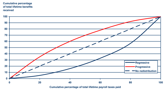
The progressivity index is constructed using Lorenz curves adapted to show the distribution of lifetime Social Security tax payments and lifetime Social Security benefit receipts. Chart 1 illustrates such curves using stylized data. Individuals are sorted by their lifetime taxes, and the horizontal axis represents the cumulative percentage of total lifetime taxes paid while the vertical axis represents the cumulative percentage of total lifetime benefits received.9 Thus, a given point on the line indicates that individuals paying x percent of total lifetime taxes receive y percent of total lifetime benefits. A line with a slope of 1, labeled as the "no-redistribution line," represents a program in which lifetime benefits are precisely proportional to lifetime taxes. A curve above the no-redistribution line represents progressivity, as it shows that individuals or households paying a given percentage of total taxes receive more than that percentage of total benefits. A curve below the no-redistribution line represents regressivity.
Progressivity of Social Security: Illustrative examples using stylized Lorenz curves
Text description for Chart 1.
Progressivity of Social Security: Illustrative examples using stylized Lorenz curves
There are three lines on the chart, labeled regressive, progressive, and no redistribution. The horizontal axis is labeled cumulative percentage of total lifetime payroll taxes paid. The vertical axis is labeled cumulative percentage of total lifetime benefits received. Both axes range from zero to 100 in increments of 20. In the chart, all three lines begin at the zero-zero coordinate and end at the 100-100 coordinate.
The no-distribution line is a straight line running from the zero-zero coordinate to the 100-100 coordinate.
The progressive and regressive lines appear as curves bending away from the no-redistribution line. The progressive line curves above the no-redistribution line and the regressive line curves below the no-distribution line. Both curves reach the maximum departure from the no-redistribution line near the 50-50 coordinate.
On the progressive line, individuals who have paid the lowest 20 percent of total taxes receive about 35 percent of the total benefits, those paying the lowest 50 percent of total taxes receive about 70 percent of the total benefits, and those paying the lowest 80 percent of the total taxes receive about 92 percent of the total benefits.
On the regressive line, individuals who have paid the lowest 20 percent of total taxes receive about 5 percent of the total benefits, those paying the lowest 50 percent of total taxes receive about 25 percent of the total benefits, and those paying the lowest 80 percent of the total taxes receive about 57 percent of the total benefits.
The curve allows for visual representation of the distribution of benefits relative to taxes. We might say, for instance, that individuals paying the bottom 20 percent of total taxes receive 35 percent of total benefits, indicating progressivity.
Moreover, from these curves a single summary measure similar to a Gini coefficient can be calculated. That summary measure—the progressivity index—is equal to the area below the curve divided by the area below the no-redistribution line, minus 1. If we label the area below the no-redistribution line A and the area below the curve B, the index value is equal to . Since area A is by definition one-half the total, this expression simplifies to . Thus, if the Lorenz curve overlaid the no-redistribution line, indicating that benefits received were precisely proportional to taxes paid, the progressivity index would equal 0. A positive index value represents progressivity while a negative index value represents regressivity.
This application of Lorenz curves and Gini coefficients resembles the Suits Index (Suits 1977), which is used to calculate the progressivity of tax payments relative to total income, although the two methods are not identical. Our approach is also similar to that of OECD (2007), which calculates the progressivity of a pension program as 1 minus the ratio of the Gini coefficient of benefits to the Gini coefficient of earnings. Our approach differs from OECD's in that first, it uses taxes rather than earnings as an input; and second, it is calculated based on lifetime taxes and benefits rather than periodic units.
Limitations and Caveats
The progressivity index can be viewed as akin to a thermometer: It provides a single measurement relative to an easily understandable scale. It is not a complete measure, just as a thermometer does not measure wind chill, humidity, or other relevant factors. Some limitations of the progressivity index are outlined below.
Given the population-level data provided by a microsimulation model or an equivalent dataset, calculating the progressivity index is fairly straightforward. However, important questions remain regarding the advantages and disadvantages of the progressivity index relative to other existing or potential approaches. Some measures of progressivity attempt to be purely descriptive; others incorporate explicit social welfare functions, such that certain outcomes can be described as "better" or "worse" than others. We make no such claims for the progressivity index.10
It must be stressed that while policy analysis of Social Security has lacked an easily applicable measure of overall system progressivity, introducing this index does not imply that other summary or disaggregated measures of progressivity should not be used. The progressivity index is designed to give an overall view of the extent of redistribution within the Social Security program and to aid analysis of how progressivity can evolve through changes in policies and the characteristics of the participant population. Other distributional outcomes are also of interest, so a variety of measures may be needed for a thorough analysis of Social Security progressivity. Moreover, all progressivity measures involve value judgments, implicit or explicit, that influence the degree of progressivity that is measured, how progressivity may be affected by changes in policy or population characteristics, and the amount of progressivity deemed desirable. The progressivity index, and the Lorenz curve/Gini coefficient approach upon which it is based, are subject to a number of criticisms, some of which follow.
The progressivity index measures the degree to which the distribution of benefits and taxes differ. Other comprehensive measures of progressivity focus on other factors. Following Musgrave and Thin (1948), many define progressivity as the degree to which a program affects the overall distribution of income.11 By this standard, the relative size of a program as an income source may be as important to its progressivity as the slant of net benefits relative to lifetime earnings. The progressivity index presented here is invariant to the scale of benefits provided. That is to say, it makes no judgment on the overall level of taxes levied or benefits provided by Social Security, but it refers only to the degree of progressivity within a given level of taxes and benefits. In practice, of course, policy decisions regarding the desired progressivity of benefits are not distinct from decisions about the average level of benefits or taxes, either from the view of public finance or that of individual social welfare. That being said, there is no clear method for gauging interactions between the level and progressivity of the tax/benefit schedules.
One reason policymakers care about progressivity in Social Security or other government programs is the assumption that lower-earning individuals derive greater welfare value from an additional dollar than do higher-earning individuals. The Gini index, or the progressivity index based on it, does not explicitly account for the diminishing marginal utility of money. As Kiefer (1984) points out, the Gini index responds to income transfers between individuals based upon their ranking in the income distribution, not upon their relative levels of income.12 Although this is clearly a limitation of both the Gini index and the progressivity index, it derives from the fact that there is no single agreed-upon social welfare function that can be applied to these questions. The Gini index is a very commonly used measure of progressivity and we believe its application here enhances understanding of Social Security redistribution, even acknowledging its limitations.
The progressivity index value is also sensitive to the distribution of earnings in the population. If, for instance, each individual had precisely the same lifetime earnings, the progressivity index would display little or no overall progressivity despite the fact that progressivity is called for in the program's benefit formula. Put another way, increases or decreases in the inequality of earnings in the population will increase or decrease measured progressivity even in the absence of policy changes. Related to the earnings distribution, our approach does not measure the effects of earnings above the current-law taxable maximum, consistent with Social Security's historical program structure of levying taxes and paying benefits only on earnings up to a cap. However, the progressivity index will account for the effects of changes in the taxable maximum, as these could affect both tax payments and benefit receipts.
Similarly, changes in household structures and other factors can alter measured progressivity. These effects can be seen in the calculations of Social Security progressivity over time: Even with constant policy parameters, progressivity changes somewhat over time due to changes in the population subject to those policies.
The index also assumes a static view of the effects of policy changes on macroeconomic variables. For instance, changes in policy could alter incentives to work or save, which would then alter lifetime earnings and benefits, or the interest rates used to discount them. These feedback effects can have additional consequences for progressivity that are not measured here.
The progressivity index differs from some other measures of progressivity in that it relates total taxes paid to total benefits received, while other measures such as Coronado, Fullerton, and Glass (2000) measure net benefits—that is, total benefits minus total taxes—as a percentage of lifetime earnings. Moreover, the Lorenz curve approach allows for easily understandable expressions of progressivity, such as taxpayers paying the bottom x percent of total taxes receiving y percent of total benefits. There is not a comparable expression based on net benefits that is as easily understandable. Likewise, the progressivity index allows for expression of overall progressivity on an understandable zero-to-one scale, which other measures may or may not be able to do.
Finally, it should be noted that the level of lifetime benefits received by individuals is a function of their longevity. Thus, as noted above, differential mortality by income could undo some of the apparent progressivity in the Social Security program. Some might argue that the effects of differential mortality should not be measured as part of system progressivity, as the annuity structure of Social Security retirement benefit provides valuable insurance against outliving one's assets and this structure could be welfare-enhancing even for individuals with lower-than-average life spans.13 However, to the degree that life expectancies differ based on a predictable and measurable factor such as lifetime earnings, Social Security's annuity structure could be altered to account for it. Thus, leaving aside the fact that most studies of Social Security's progressivity do include the effect of differential mortality, ignoring the effects of predictable mortality differences on lifetime benefits would eliminate information potentially useful to policymakers. This serves as a reminder that an explicit social welfare function may produce different results from the progressivity index presented here.
Using the MINT Model to Analyze Progressivity
The progressivity index requires individual-level data that provide a representative population. SSA's Modeling Income in the Near Term (MINT) model is particularly useful for this purpose. It projects demographic changes, lifetime earnings, and retirement income of future retirees, while accounting for the heterogeneity of mortality, household formation and dissolution, relative earnings between spouses, and numerous other social and economic changes (for example, real growth in economy-wide earnings between cohorts) that affect the taxes paid to and expected benefits received from Social Security.
MINT was developed by SSA's Office of Research, Evaluation, and Statistics with assistance from the Brookings Institution, the RAND Corporation, and the Urban Institute. Its projections are based on observed data from the U.S. Census Bureau's Survey of Income and Program Participation (SIPP) 1990–1993 and 1996 panels, which are matched to SSA earnings, benefit, and mortality records.14 In this paper, we use data from MINTEX, an extended model combining data from MINT versions 3 and 4, which is built on the assumptions chosen by the Board of Trustees and used by SSA's Office of the Chief Actuary (OCACT) to estimate Social Security's finances in the 2004 Social Security Trustees Report (Board of Trustees 2004).15 The model projects 231,000 individuals through 2099 and captures demographic and economic changes both between and within birth cohorts, such as marital patterns, race/ethnicity, mortality, labor force attachment, educational attainment, earnings patterns, and immigration.
While a thorough exposition of MINT's projection methodology goes beyond the scope of this paper, the earnings and age distributions in the birth cohorts play key roles in determining the progressivity index's results and require some explanation. Earnings projections are based on matched data derived from SSA's Summary Earnings Record (SER) from 1951 to 2001. Using an "earnings splicing" approach, the observed earnings of an older worker (the donor individual) are spliced onto the incomplete earning records of a worker in a younger cohort (the target individual). This approach also integrates mortality into the projections, which helps shape the age structure of each cohort.16 The donor and target individuals are determined via a hot-deck imputation that statistically matches targets with donors based on a number of categories, including demographic characteristics, educational attainment, and earnings history.17 The hot-deck method thereby allows for expected demographic and economic differences between cohorts. However, it does not account for possible future changes in relationships between earnings and the factors used to find the nearest neighbor, such as education. Detailed documentation of the MINT model can be found in Toder and others (2002) and Smith, Cashin, and Favreault (2005).
The MINT population characteristics are also calibrated to reflect increases in life expectancy for future generations. Mortality estimates are derived from gender- and age-specific rates based on the 2004 Trustees' assumptions through age 66. After this age, mortality projections essentially follow a hazard model outlined in chapter 8 of Toder and others (2002). For the extended cohorts (1973–2017), mortality prior to age 65 was also adjusted to meet the 2004 Trustees' assumptions. Adjustment factors were added from estimated regressions of the age- and cohort-specific life expectancy (Smith, Cashin, and Favreault 2005, chapter 5).
MINTEX extends the population beyond its original "near term" structure to include the 1973–2017 birth cohorts. MINTEX uses Current Population Survey (CPS) data and Census projections to match target individuals to a donor population from the 1960–1964 cohort in MINT 4.18 The same earnings splicing and hot-deck methodologies were applied. While these younger cohorts are projected based on observed earning patterns of those "nearest neighbors" born in 1960–1964, again, the selective nature of the hot decking builds in expected cross-cohort differences in demographics, labor force attachment of women, earnings patterns, mortality, and other characteristics.
Overall, MINT is a comprehensive, robust database of individual earnings and demographic information that can be used to project the effects of Social Security policy changes on retirement income and poverty statistics across birth cohorts.19 Like any microsimulation model, however, MINT has several noteworthy limitations. One is that MINT does not fully account for immigration, particularly in the extended or imputed cohorts. Another issue is that the retirement behavior, along with demographic and other economic characteristics of previous cohorts, is inferred to extended cohorts (1973–2017). As a result, estimates for these birth cohorts are less reliable than those for retirees from observed birth cohorts. That is to say, to the extent that certain relationships change in new birth cohorts, such as labor force participation rates, marriage rates, longevity, and changes in pensions, the projections for the imputed cohorts will need to be revisited.
Methodological Choices
We make a number of simplifying methodological decisions that influence the results. First, our analysis begins with the application of the progressivity index to nondisabled individuals born between 1941 and 1945 and who are alive at ages 62–66 in 2007. We use nondisabled individuals because their lifetime earnings patterns are different enough from the disabled that it appears to be appropriate to examine progressivity for the retirement and disability elements of the Social Security program distinctly. The decision to restrict our analysis to those who survive to retirement will increase measured progressivity, as individuals who die prior to retirement have lower lifetime earnings and lower benefit receipts than retirees. While analysis is warranted of individuals who die prior to claiming benefits, and also of any household members who may be eligible for survivor benefits, we believe that in this instance restricting to those who survive to retirement age is consistent with the social insurance nature of the program.
Second, we use observed lifetime Old-Age, Survivors, and Disability Insurance (OASDI) benefits and taxes. We limit the analysis to nondisabled individuals, however those individuals can be married to disabled workers who provide aged spousal and survivor benefits based on disability contributions. Also, those disabled spouses may convert to retirement benefits. As noted below, the shared nature of the analysis means that spouse's benefits and taxes are taken into account during the course of each marriage. Income taxes on benefits were not estimated because at this point MINT does not provide enough information to adequately calculate adjusted gross income for retirees.
Third, we use the shared approach to calculate the present value of lifetime benefits and taxes. The shared approach averages the observed benefits and taxes for a couple in each year they are married, and thereby controls for differences in household structure and for earnings inequality between spouses. This approach will tend to reduce measured progressivity, as it does not measure actual redistribution between higher- and lower-earning members of the same household. This seems appropriate, however, if we assume that spouses tend to share the burdens and benefits of participation in the Social Security program.
Fourth, we base our analysis on the individual's shared OASDI tax payments, not on the individual's shared earnings, either in total or subject to the payroll tax ceiling. In part, this is to be consistent with the historical structure of the program, which has calculated taxes and benefits based on wages up to a given maximum. As long as the payroll tax is levied on a flat basis, tax payments will be proportional to earnings subject to payroll taxes. The choice to measure progressivity relative to taxes rather than uncapped earnings will increase measured progressivity, since it omits untaxed wages of earnings above the ceiling. In this sense, the progressivity index does not focus on an "ability to pay" basis. However, using tax payments in the progressivity index allows measured progressivity to change if the payroll tax is levied in a progressive fashion or if the maximum taxable wage is changed. This provides additional flexibility for policy analysis.
Fifth, we discount benefits and taxes at the effective interest rate earned by the Social Security trust funds; for future years, the intermediate projection from the 2004 Social Security Trustees Report is used. The choice of interest rate series can affect the distributional results. A lower discount rate could be justified if we believe that the Social Security program overcomes inefficiencies in private markets, such as the absence of insurance against low lifetime wages or adverse selection in annuity markets. A higher interest rate could be justified based on the political risk of the program, particularly given future funding shortfalls. In experiments using the high or low projected interest rate values from the Social Security Trustees Report (Board of Trustees 2004), effects on measured progressivity were modest.20
To maintain equivalence between the different birth cohorts used in the analysis, lifetime taxes and benefits are first computed on a present value basis as of age 62, then wage indexed to a common year. This process prevents distortions in the results caused by the increase in average wages from cohort to cohort.
Progressivity of Social Security for Recent Retirees
The results for the 1941–1945 birth cohort are displayed in Chart 2. Chart 2 shows that individuals paying the bottom 50 percent of total taxes receive roughly 61 percent of total benefits. The progressivity index value under current law for individuals born between 1941 and 1945 is 0.16. In our view, this indicates that Social Security is modestly progressive between above-average and below-average lifetime earners. Characterizing a given level of progressivity as modest or otherwise is a subjective judgment. To help in making these judgments the following section provides several stylized benchmarks.
Progressivity of Social Security for recent retirees: Lorenz Curve for 1941–1945 birth cohort members who survive to claim retirement benefits
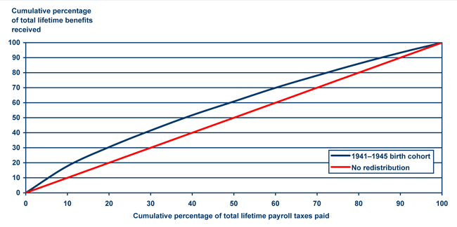
Text description for Chart 2.
Progressivity of Social Security for recent retirees: Lorenz Curve for 1941–1945 birth cohort members who survive to claim retirement benefits
There are two lines on the chart, labeled 1941–1945 birth cohort and no redistribution. The horizontal axis is labeled cumulative percentage of total lifetime payroll taxes paid. The vertical axis is labeled cumulative percentage of total lifetime benefits received. Both axes range from zero to 100 in increments of 10. In the chart, both lines begin at the zero-zero coordinate and end at the 100-100 coordinate.
The no-redistribution line is a straight line running from the zero-zero coordinate to the 100-100 coordinate.
The 1941–1945 birth cohort line appears as a curve bending above the no-redistribution line, with a maximum departure from the no-redistribution line near the 40-40 coordinate.
On the 1941–1945 birth cohort line, individuals who have paid the lowest 20 percent of total taxes receive about 30 percent of the total benefits, those paying the lowest 40 percent of total taxes receive about 52 percent of the total benefits, those paying the lowest 60 percent of taxes receive about 70 percent of total benefits, and those paying the lowest 80 percent of the total taxes receive about 86 percent of the total benefits.
Progressivity under Current Law in Comparison with Two Stylized Programs
While the no-redistribution line noted in the preceding section provides some context with which to understand whether the program is progressive, it is helpful to compare the program with more intuitive examples along the progressivity continuum. For this reason, we compare the index values for current law to two stylized policies designed to illustrate intuitive "book-ends" of progressivity. The first is a flat-dollar annuity payment in which each individual receives the same periodic benefit payment regardless of pre-retirement earnings; this flat-dollar benefit is similar to a "universal pension" as employed in several developing countries.21 The second is a pure defined contribution (DC) program in which each individual receives a lump sum at retirement based on the investment of a percentage of his or her earnings when employed. This lump sum is assumed not to be annuitized.
Chart 3 illustrates the progressivity curves for a flat-dollar benefit and for a pure DC program.22 The flat-dollar benefit should be considerably more progressive than the current benefit schedule, whose equity provisions increase total benefits based on prior earnings. Under the flat-dollar benefit, replacement rates and internal rates of return would be an inverse function of earnings, as increases in earnings would not produce any increase in benefits. The progressivity curve bears this out, lying well above that for current-law Social Security. Under the flat-dollar benefit approach, individuals paying the bottom 50 percent of total taxes would receive 71 percent of total benefits, versus 61 percent under Social Security. Likewise, the flat-dollar benefit produces a progressivity index value of 0.33, compared with 0.16 for the current-law Social Security program.
Progressivity of Social Security compared with stylized alternatives: Lorenz curves for flat-dollar benefit, current-law Social Security, and defined contribution (DC) plan for 1941–1945 birth cohort members who survive to claim retirement benefits
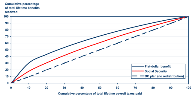
Text description for Chart 3.
Progressivity of Social Security compared with stylized alternatives: Lorenz curves for flat-dollar benefit, current-law Social Security, and defined contribution (DC) plan for 1941–1945 birth cohort members who survive to claim retirement benefits
There are three lines on the chart, labeled flat-dollar benefit, Social Security, and defined contribution (DC) plan, which is equivalent to no redistribution. The horizontal axis is labeled cumulative percentage of total lifetime payroll taxes paid. The vertical axis is labeled cumulative percentage of total lifetime benefits received. Both axes range from zero to 100 in increments of 10. In the chart, all three lines begin at the zero-zero coordinate and end at the 100-100 coordinate.
The DC plan line is a straight line running from the zero-zero coordinate to the 100-100 coordinate.
The flat-dollar benefit and Social Security lines both appear as curves bending above the DC plan line. The flat-dollar benefit curve reaches the maximum departure from the DC plan line near the 10-10 coordinate, and the Social Security curve reaches the maximum departure from the DC plan line near the 40-40 coordinate.
On the flat-dollar benefit line, individuals who have paid the lowest 10 percent of total taxes receive about 30 percent of the total benefits, those paying the lowest 50 percent of total taxes receive about 70 percent of the total benefits, and those paying the lowest 80 percent of the total taxes receive about 90 percent of the total benefits.
On the Social Security line, individuals who have paid the lowest 10 percent of total taxes receive about 18 percent of the total benefits, those paying the lowest 50 percent of total taxes receive about 60 percent of the total benefits, and those paying the lowest 80 percent of the total taxes receive about 85 percent of the total benefits.
Chart 3 also shows the progressivity curve for the pure DC program. This method should be less progressive than the current system, as it contains none of the current benefit formula's progressive provisions. The DC curve in Chart 3 lies precisely on the no-redistribution line and produces a progressivity index score of zero.
Although the comparison is not straightforward given the possibility that progressivity follows a non-linear function, the current-law progressivity index value of 0.16 lies roughly halfway between a flat dollar benefit value of 0.33 and a pure DC program value of zero. This comparison demonstrates the ability of the progressivity index to show not only absolute levels of progressivity but also the differences between different benefit formulas or between different populations in a relatively simple and understandable way.
Progressivity among Future Cohorts of Retirees
In addition to estimating progressivity under Social Security for current retirees, MINT data can project progressivity among future participant cohorts. This is of interest because it shows how progressivity index values can be altered by changes in the underlying participant population rather than through changes in policy. Lifetime Social Security taxes and retirement benefits are affected by a variety of socioeconomic and demographic factors, including interest rates, the economy-wide distribution of earnings, differential mortality, age-earnings profiles, household composition and marriage patterns, and the relative earnings between spouses. Changes in any or all of these factors may change the effective progressivity of the program over time, even in the absence of significant policy changes.
To illustrate, we calculate the progressivity index for individuals born in 5-year spans from 1926 through 2017 (those cohorts who reach age 67 between 1993 and 2084).23 Chart 4 reports progressivity index results for these cohorts on the 0 to 1 scale, showing the progressivity trend projected by MINT across cohorts. The progressivity index of Social Security retirement benefits will decline from just under 0.24 for those born 1926–1930 to about 0.15 for those born 1946–1950 and later. Stated differently, the progressivity of the Social Security program drops substantially for cohorts retiring in the mid- and late 2010s, but then remains roughly constant in following years.
Progressivity index of current-law Social Security benefits by birth cohort
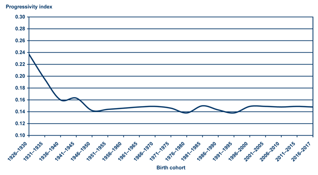
| Birth cohort | Current law progressivity index |
|---|---|
| 1926–1930 | 0.237 |
| 1931–1935 | 0.195 |
| 1936–1940 | 0.160 |
| 1941–1945 | 0.163 |
| 1946–1950 | 0.142 |
| 1951–1955 | 0.144 |
| 1956–1960 | 0.146 |
| 1961–1965 | 0.148 |
| 1966–1970 | 0.149 |
| 1971–1975 | 0.146 |
| 1976–1980 | 0.138 |
| 1981–1985 | 0.150 |
| 1986–1990 | 0.143 |
| 1991–1995 | 0.138 |
| 1996–2000 | 0.149 |
| 2001–2005 | 0.149 |
| 2006–2010 | 0.148 |
| 2011–2015 | 0.149 |
| 2016–2017 | 0.148 |
Chart 5 and Table 1 provide greater detail, showing the percentage of total benefits received broken down by lifetime earnings deciles for individuals paying taxes. For instance, Chart 5 and Table 1 show that in the 1926–1930 birth cohort, individuals paying the bottom 10 percent of total lifetime payroll taxes received 22.2 percent of total lifetime benefits. For the 1956–1960 birth cohort, total benefits received by individuals paying the bottom 10 percent of taxes are projected to decline to 17.0 percent and remain at that level for later cohorts. As shown in Table 2, the decline in progressivity appears to take place primarily in the bottom three deciles of taxpayers, where the share of total benefits received declines over time. From the 4th through 10th deciles of taxpayers, the share of total benefits received increases between the 1926–1930 and 1951–1955 birth cohorts. The largest increase in relative benefits occurs in the 9th decile of taxpayers, whose relative share of total benefits rises by 29 percent between the 1926–1930 and 2016–2017 birth cohorts.
Cumulative percentage of total lifetime benefits received by individuals below selected deciles of shared lifetime earnings distribution, by birth cohort
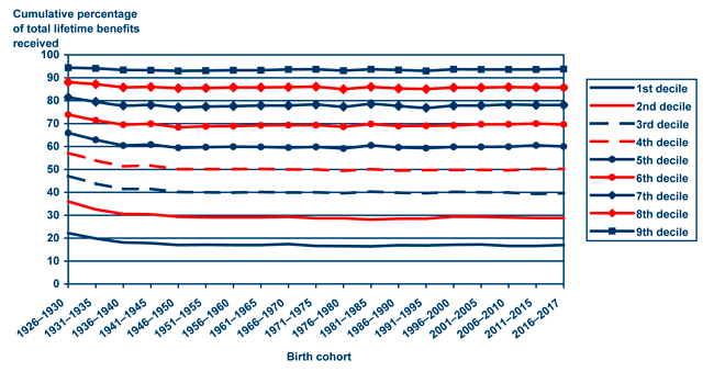
| Birth cohort | 1st decile | 2nd decile | 3rd decile | 4th decile | 5th decile | 6th decile | 7th decile | 8th decile | 9th decile |
|---|---|---|---|---|---|---|---|---|---|
| 1926–1930 | 22.2 | 36.0 | 47.2 | 57.2 | 65.9 | 73.9 | 81.4 | 88.1 | 94.4 |
| 1931–1935 | 19.8 | 32.5 | 43.8 | 53.9 | 62.9 | 71.4 | 79.5 | 87.2 | 94.1 |
| 1936–1940 | 18.1 | 30.5 | 41.4 | 51.3 | 60.4 | 69.5 | 77.9 | 85.8 | 93.4 |
| 1941–1945 | 17.8 | 30.4 | 41.5 | 51.7 | 60.8 | 69.9 | 78.1 | 86.0 | 93.3 |
| 1946–1950 | 17.0 | 29.3 | 40.1 | 50.1 | 59.4 | 68.4 | 77.1 | 85.4 | 93.0 |
| 1951–1955 | 17.1 | 29.1 | 40.0 | 50.1 | 59.7 | 68.8 | 77.4 | 85.5 | 93.1 |
| 1956–1960 | 17.0 | 29.1 | 39.9 | 50.1 | 59.9 | 68.9 | 77.6 | 85.8 | 93.3 |
| 1961–1965 | 17.0 | 29.1 | 40.1 | 50.2 | 59.8 | 69.2 | 77.9 | 85.8 | 93.3 |
| 1966–1970 | 17.4 | 29.3 | 39.9 | 50.0 | 59.5 | 69.3 | 77.9 | 85.9 | 93.6 |
| 1971–1975 | 16.6 | 28.7 | 40.0 | 50.0 | 59.8 | 69.3 | 78.3 | 86.1 | 93.7 |
| 1976–1980 | 16.5 | 28.7 | 39.6 | 19.4 | 59.1 | 68.6 | 77.4 | 85.0 | 93.1 |
| 1981–1985 | 16.4 | 28.1 | 40.3 | 50.1 | 60.5 | 69.8 | 78.5 | 86.0 | 93.7 |
| 1986–1990 | 16.9 | 28.5 | 39.8 | 49.5 | 59.6 | 68.9 | 77.7 | 85.3 | 93.4 |
| 1991–1995 | 16.8 | 28.5 | 39.6 | 49.7 | 59.3 | 69.0 | 76.9 | 85.1 | 93.0 |
| 1996–2000 | 17.1 | 29.4 | 40.2 | 49.8 | 59.8 | 69.2 | 77.8 | 85.7 | 93.7 |
| 2001–2005 | 17.2 | 29.3 | 40.0 | 49.8 | 59.8 | 69.7 | 77.9 | 85.7 | 93.6 |
| 2006–2010 | 16.6 | 29.0 | 39.9 | 49.6 | 59.9 | 69.7 | 78.3 | 85.9 | 93.6 |
| 2011–2015 | 16.6 | 28.8 | 39.3 | 50.2 | 60.5 | 70.0 | 78.1 | 85.8 | 93.6 |
| 2016–2017 | 17.0 | 28.8 | 39.6 | 50.2 | 60.0 | 69.6 | 78.1 | 85.7 | 93.8 |
| Birth cohort | Cumulative percentage of total benefits received by decile of total taxes paid | |||||||||
|---|---|---|---|---|---|---|---|---|---|---|
| 1st | 2nd | 3rd | 4th | 5th | 6th | 7th | 8th | 9th | 10th | |
| 1926–1930 | 22.2 | 36.0 | 47.2 | 57.2 | 65.9 | 73.9 | 81.4 | 88.1 | 94.4 | 100.0 |
| 1931–1935 | 19.8 | 32.5 | 43.8 | 53.9 | 62.9 | 71.4 | 79.5 | 87.2 | 94.1 | 100.0 |
| 1936–1940 | 18.1 | 30.5 | 41.4 | 51.3 | 60.4 | 69.5 | 77.9 | 85.8 | 93.4 | 100.0 |
| 1941–1945 | 17.8 | 30.4 | 41.5 | 51.7 | 60.8 | 69.9 | 78.1 | 86.0 | 93.3 | 100.0 |
| 1946–1950 | 17.0 | 29.3 | 40.1 | 50.1 | 59.4 | 68.4 | 77.1 | 85.4 | 93.0 | 100.0 |
| 1951–1955 | 17.1 | 29.1 | 40.0 | 50.1 | 59.7 | 68.8 | 77.4 | 85.5 | 93.1 | 100.0 |
| 1956–1960 | 17.0 | 29.1 | 39.9 | 50.1 | 59.9 | 68.9 | 77.6 | 85.8 | 93.3 | 100.0 |
| 1961–1965 | 17.0 | 29.1 | 40.1 | 50.2 | 59.8 | 69.2 | 77.9 | 85.8 | 93.3 | 100.0 |
| 1966–1970 | 17.4 | 29.3 | 39.9 | 50.0 | 59.5 | 69.3 | 77.9 | 85.9 | 93.6 | 100.0 |
| 1971–1975 | 16.6 | 28.7 | 40.0 | 50.0 | 59.8 | 69.3 | 78.3 | 86.1 | 93.7 | 100.0 |
| 1976–1980 | 16.5 | 28.7 | 39.6 | 49.4 | 59.1 | 68.6 | 77.4 | 85.0 | 93.1 | 100.0 |
| 1981–1985 | 16.4 | 28.1 | 40.3 | 50.1 | 60.5 | 69.8 | 78.5 | 86.0 | 93.7 | 100.0 |
| 1986–1990 | 16.9 | 28.5 | 39.8 | 49.5 | 59.6 | 68.9 | 77.7 | 85.3 | 93.4 | 100.0 |
| 1991–1995 | 16.8 | 28.5 | 39.6 | 49.7 | 59.3 | 69.0 | 76.9 | 85.1 | 93.0 | 100.0 |
| 1996–2000 | 17.1 | 29.4 | 40.2 | 49.8 | 59.8 | 69.2 | 77.8 | 85.7 | 93.7 | 100.0 |
| 2001–2005 | 17.2 | 29.3 | 40.0 | 49.8 | 59.8 | 69.7 | 77.9 | 85.7 | 93.6 | 100.0 |
| 2006–2010 | 16.6 | 29.0 | 39.9 | 49.6 | 59.9 | 69.7 | 78.3 | 85.9 | 93.6 | 100.0 |
| 2011–2015 | 16.6 | 28.8 | 39.3 | 50.2 | 60.5 | 70.0 | 78.1 | 85.8 | 93.6 | 100.0 |
| 2016–2017 | 17.0 | 28.8 | 39.6 | 50.2 | 60.0 | 69.6 | 78.1 | 85.7 | 93.8 | 100.0 |
| SOURCE: Authors’ calculations using Modeling Income in the Near Term (MINT) data. | ||||||||||
| Decile of total taxes paid | 1951–1955 cohort share as percentage of 1926–1930 cohort share | 2016–2017 cohort share as percentage of 1926–1930 cohort share |
|---|---|---|
| 1st | 77.0 | 76.6 |
| 2nd | 87.0 | 85.5 |
| 3rd | 97.3 | 96.4 |
| 4th | 101.0 | 106.0 |
| 5th | 110.3 | 112.6 |
| 6th | 113.8 | 120.0 |
| 7th | 114.7 | 113.3 |
| 8th | 120.9 | 113.4 |
| 9th | 120.6 | 128.6 |
| 10th | 123.2 | 110.7 |
| SOURCE: Authors’ calculations using Modeling Income in the Near Term (MINT) data. | ||
Several factors may affect how changing household structures, and the auxiliary benefits they produce, influence the progressivity of the Social Security program.24 On one hand, assortative pairing among individuals paying higher total taxes could reduce the payment of auxiliary benefits within these households, as they would have similar lifetime earnings.25 On the other hand, individuals paying the lowest total taxes may increasingly come to be those who never married, and therefore are also ineligible for auxiliary benefits. Thus, it is not clear before the fact how changes in household structures and earnings will impact auxiliary benefit payments.
To shed additional light, Chart 6 shows progressivity index figures for Social Security, isolating worker benefits (based on an individual's own earnings record) and auxiliary benefits (based on the earnings record of a spouse). Note that in both cases, shared taxes continue to be used in calculating the progressivity index. Chart 6 shows several interesting results. First, auxiliary benefits are significantly more progressive than worker benefits, even when measured on a shared basis that accounts for a higher-earning spouse whose earnings record generated the auxiliary benefits. For the 1926–1930 birth cohort, for instance, the progressivity index value for auxiliary benefits is 0.48, significantly higher than the 0.33 index value for a flat-dollar benefit. The progressivity index value for earned benefits for the same cohort, by contrast, is only 0.21. This is because the largest relative auxiliary benefits can be paid to a household in which one spouse does not work, which in turn limits the total earnings of the household.26
Progressivity indices for Social Security auxiliary and work benefits, by birth cohort
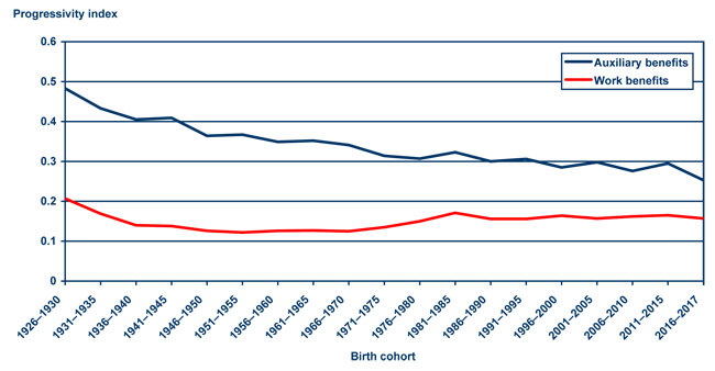
| Birth cohort | Auxiliary benefits | Work benefits |
|---|---|---|
| 1926–1930 | 48.3 | 20.7 |
| 1931–1935 | 43.3 | 16.9 |
| 1936–1940 | 40.5 | 14.0 |
| 1941–1945 | 40.9 | 13.8 |
| 1946–1950 | 36.4 | 12.6 |
| 1951–1955 | 36.7 | 12.2 |
| 1956–1960 | 34.9 | 12.6 |
| 1961–1965 | 35.2 | 12.7 |
| 1966–1970 | 34.1 | 12.5 |
| 1971–1975 | 31.4 | 13.5 |
| 1976–1980 | 30.7 | 15.0 |
| 1981–1985 | 32.3 | 17.1 |
| 1986–1990 | 30.0 | 15.6 |
| 1991–1995 | 30.6 | 15.6 |
| 1996–2000 | 28.5 | 16.4 |
| 2001–2005 | 29.8 | 15.7 |
| 2006–2010 | 27.6 | 16.2 |
| 2011–2015 | 29.5 | 16.5 |
| 2016–2017 | 25.3 | 15.7 |
Second, the progressivity of auxiliary benefits is projected to decline significantly more than the progressivity of worker benefits. For the 1926–1930 birth cohort, the progressivity index value for auxiliary benefits is about 0.27 higher than for worker benefits, but for the 1966–1970 birth cohort the projected difference is 0.21, and for the 1996–2000 birth cohort the projected difference is only 0.12. Likely causes are a general decline in the disparity between spouses' earnings, thus reducing the relative generosity of auxiliary benefits; and the increase in the share of divorced or never-married individuals reaching retirement age, reducing the share of individuals eligible for spouse, or more typically survivor, benefits.27 This decline is not enough, however, to greatly reduce the long-run progressivity of Social Security as a whole. Auxiliary benefits, net of the worker benefits to which an individual would otherwise be entitled, are a relatively small share of total benefits. In the future, net auxiliary benefits are projected to diminish further as women's lifetime earnings more closely resemble those of men, resulting in fewer women being eligible for spouse benefits and in smaller widow(er)s benefits relative to the total household benefits received when both spouses were alive.28
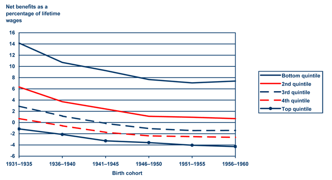
The projected decline in progressivity from the 1926–1930 through 1946–1950 birth cohorts differs from some previous studies on progressivity. For example, using MINT data, Smith, Toder, and Iams (2003) concluded that progressivity would increase for the 1956–1960 cohorts compared with those born between 1931 and 1935, in part because of increased women's labor force participation.29 Chart 7 illustrates that ratios of the present value of benefits net of taxes to lifetime earnings decline over time for all lifetime earnings quintiles save the bottom quintile. This appears to justify the conclusion, contrary to that found using the progressivity index, that progressivity in the Social Security retirement program will tend to increase rather than decrease over time.
Net benefits as a percentage of lifetime wages by birth cohort and earnings quintile
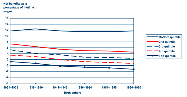
| Birth cohort | Bottom quintile | 2nd quintile | 3rd quintile | 4th quintile | Top quintile |
|---|---|---|---|---|---|
| 1931–1935 | 11.7 | 7.3 | 5.3 | 3.5 | 1.3 |
| 1936–1940 | 12.4 | 6.4 | 4.1 | 3.0 | 0.7 |
| 1941–1945 | 11.7 | 5.5 | 3.6 | 2.0 | -0.2 |
| 1946–1950 | 11.5 | 5.0 | 2.8 | 1.3 | -0.6 |
| 1951–1955 | 11.5 | 4.9 | 2.7 | 1.0 | -0.8 |
| 1956–1960 | 11.7 | 4.5 | 2.4 | 0.7 | -1.3 |
The different results are initially difficult to explain, given that they derive from very similar data sources and that definitions of progressivity used in both appear intuitively plausible. Although the different results may have additional methodological sources, we believe the greatest difference derives from the samples of individuals examined in each approach. Our analysis focuses on the retirement portion of Social Security and restricts itself to individuals who survive to claim benefits and who never received Disability Insurance (DI) benefits. While Smith, Toder, and Iams also exclude DI benefits from their calculations, their population includes retirement beneficiaries who initially qualified for benefits as disabled workers. Under current law, individuals receiving DI payments transfer to Old-Age Insurance payments upon reaching the normal retirement age. Thus, a nonrestricted sample of OASI beneficiaries would include a certain percentage of individuals who initially qualified for benefits under the DI program. The disabled tend to have low lifetime earnings and payroll contributions due to separation from the labor force. In addition, the disability benefit formula has a truncated benefit computation period that does not penalize a disabled individual, as it would a similarly lower-earning nondisabled individual who simply had low labor-force attachment.
If the percentage of OASI beneficiaries whose initial entitlement came through the DI program increases, this could alter the measured progressivity of the program over time. Chart 8, based on MINT data, shows the percentage of Old-Age Insurance beneficiaries in each birth cohort who initially claimed benefits through the DI program. For the earliest age cohorts this share was very small, in part because DI benefits were not available until the 1950s. For later birth cohorts, however, the availability of DI benefits, the loosening of qualification standards in the 1980s,30 and the increasing life expectancy of disabled individuals resulted in greater shares of retirees who initially received benefits as disabled workers. For the 1956–1960 birth cohort, MINT projects that 8.6 percent of retirees were initially disabled. In later cohorts this percentage is projected to rise even further. Significantly, it is likely that a disproportionate share of these former DI beneficiaries would reside in the lower end of the tax-paying distribution.
Percentage of retirees who claimed Disability Insurance benefits prior to retirement, by selected birth cohort
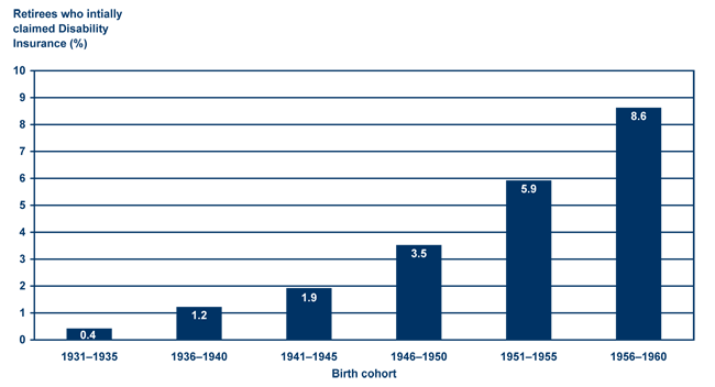
| Birth cohort | Percent |
|---|---|
| 1931–1935 | 0.4 |
| 1936–1940 | 1.2 |
| 1941–1945 | 1.9 |
| 1946–1950 | 3.5 |
| 1951–1955 | 5.9 |
| 1956–1960 | 8.6 |
Chart 9 recreates the Smith, Toder, and Iams data shown in Chart 7, but omits individuals who claimed disability benefits prior to retirement. The exclusion of the disabled lowers net benefit ratios on average. More significantly, however, the decline in net benefit ratios over time is steepest for individuals in the bottom two quintiles of lifetime earnings. It therefore appears that the maintenance of net benefit ratios for low earners in Smith, Toder, and Iams may not solely result from changing household structures and female labor force participation, as the authors conclude, but also relates to increases in the number of disabled individuals transferring to the Social Security retirement program. This appears to reconcile the Smith, Toder, and Iams findings with the results of the progressivity index shown in Chart 4. Although the retirement portion of the Social Security program appears to have become less progressive over the last several decades, the combined Social Security program may have become more progressive due to increases in the share of total beneficiaries claiming highly progressive DI program benefits.
Net benefits as a percentage of lifetime wages for nondisabled retirees, by birth cohort and earnings quintile
| Birth cohort | Bottom quintile | 2nd quintile | 3rd quintile | 4th quintile | Top quintile |
|---|---|---|---|---|---|
| 1931–1935 | 14.16235 | 6.337606 | 2.921391 | 0.706645 | -1.14279 |
| 1936–1940 | 10.71107 | 3.714741 | 1.150446 | -0.58548 | -2.12479 |
| 1941–1945 | 9.257679 | 2.41852 | -0.15368 | -1.74587 | -3.26489 |
| 1946–1950 | 7.663261 | 1.114125 | -1.07747 | -2.37612 | -3.58096 |
| 1951–1955 | 7.065951 | 0.945317 | -1.435 | -2.51094 | -4.0481 |
| 1956–1960 | 7.389889 | 0.692422 | -1.41233 | -2.6444 | -4.28859 |
Changes in Progressivity Resulting from Policy Changes
The Social Security program faces a long-term funding shortfall as the American population ages. A number of policies have been proposed to help address this shortfall. While these policies aim principally to alter the relative levels of taxes and benefits for future cohorts of participants, many would also change the distribution of taxes and benefits. There are many ways to evaluate the impact of policy options on Social Security progressivity. In this paper, we illustrate how the progressivity index can be used to compare changes to the progressivity of Social Security under a number of policy changes.
For illustrative purposes, we use policy options described by the Social Security Advisory Board (2005), which outlines a "menu" of potential changes to educate policymakers and the public on the most common proposals to address the Social Security financing shortfall. Some of these changes would have limited distributional effects as measured by the progressivity index, such as increases in the payroll tax rate or the normal retirement age, which tend to affect individuals in uniform ways across the earnings distribution.
Other changes would have distinct distributional effects that can alter Social Security’s progressivity. While necessarily selective, and with the caveat that these policies are not equivalent in the degree to which they alter Social Security's system financing, the progressivity index for Social Security is calculated under three potential changes:
- Increase the maximum taxable wage so that 90 percent of covered earnings are subject to taxation (Tax max 90) beginning in 2008. Doing so would subject a greater share of high earners' total wages to payroll taxes and would pay benefits at retirement based on those higher wages. Making this change would tend to increase progressivity, as the additional benefits are unlikely to be equal in present value to the additional taxes paid.
- Increase the number of work years used to calculate benefits to 38 (38 comp yrs). Currently, Social Security retirement benefits are based on the 35 highest-earning years in an individual's working lifetime. Increasing the computation period beginning in 2006 would tend to reduce benefits more for individuals with low lifetime earnings, since these individuals have fewer average years of covered employment. This would tend to reduce progressivity, but since many low lifetime earners who are disabled or survivors would be protected, the reduction is slight.
- Use progressive indexing (PI) for future benefits. Inflation-adjusted benefits for lifetime maximum taxable wage earners would be frozen beginning in 2012, while scheduled (wage-indexed) retirement benefits would be paid to earners in the bottom 30 percent of the earnings distribution. Individuals between the 30th and 100th percentiles of the earnings distribution would receive a mix of wage- and price-indexed initial benefits. This change would tend to increase progressivity, as initial benefits for high earners would increase at a slower rate from cohort to cohort than would benefits for lower earners.
For each policy change, we calculate the progressivity index for retirees born from 1926 to 2017 who live at least to age 62 and are never disabled. This allows for the change to be fully implemented and to be applied to future cohorts of retirees, as intended, rather than only to current participants. The results are shown in Chart 10.
Progressivity indices of current-law Social Security benefits and 3 alternative policy options, by birth cohort
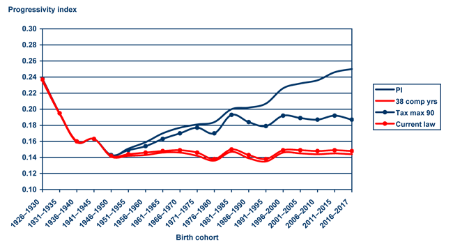
| Birth cohort | PI | 38 comp yrs | Tax max 90 | Current law |
|---|---|---|---|---|
| 1926–1930 | 0.235 | 0.235 | 0.238 | 0.237 |
| 1931–1935 | 0.194 | 0.194 | 0.195 | 0.195 |
| 1936–1940 | 0.159 | 0.159 | 0.160 | 0.160 |
| 1941–1945 | 0.163 | 0.163 | 0.163 | 0.163 |
| 1946–1950 | 0.142 | 0.141 | 0.143 | 0.142 |
| 1951–1955 | 0.151 | 0.142 | 0.149 | 0.144 |
| 1956–1960 | 0.159 | 0.143 | 0.154 | 0.146 |
| 1961–1965 | 0.170 | 0.146 | 0.163 | 0.148 |
| 1966–1970 | 0.177 | 0.146 | 0.170 | 0.149 |
| 1971–1975 | 0.181 | 0.142 | 0.177 | 0.146 |
| 1976–1980 | 0.184 | 0.136 | 0.170 | 0.138 |
| 1981–1985 | 0.200 | 0.147 | 0.193 | 0.150 |
| 1986–1990 | 0.202 | 0.139 | 0.184 | 0.143 |
| 1991–1995 | 0.207 | 0.135 | 0.179 | 0.138 |
| 1996–2000 | 0.226 | 0.146 | 0.192 | 0.149 |
| 2001–2005 | 0.232 | 0.145 | 0.189 | 0.149 |
| 2006–2010 | 0.236 | 0.144 | 0.187 | 0.148 |
| 2011–2015 | 0.246 | 0.145 | 0.192 | 0.149 |
| 2016–2017 | 0.250 | 0.144 | 0.187 | 0.148 |
The increase in the benefit computation period from 35 to 38 years has a slightly negative effect on progressivity, as expected. However, the effect is modest relative to the effects of the other policy changes, as the progressivity index would drop only from 0.149 to 0.146 for those born between 1996 and 2000 under this option.
Both progressive indexing and raising the taxable maximum wage would increase Social Security's progressivity. Progressive indexing would be only slightly more progressive than raising the taxable maximum for those born 1986–1990 (with scores of 0.20 and 0.18, respectively). However, the difference between the two widens as progressive indexing asymptotically approaches a flat benefit for all worker beneficiaries over the 30th percentile of the lifetime earnings distribution. For the 2016–2017 birth cohort the progressivity of current-law Social Security would be about 0.15. For context, the progressivity index value for the pure DC plan was zero while for a flat-dollar benefit the index value was 0.33. Raising the taxable maximum would increase progressivity to 0.19. The effects of progressive indexing would be even more substantial: Its long-term progressivity index value would be 0.25, making the program's net redistribution more closely resemble a flat-dollar benefit. Needless to say, this is taking an extremely long view on distributional analysis, but it does provide some indication of the extent to which potential changes could alter the allocation of taxes and benefits as they become fully implemented or reach a steady state.31
It is important to note that a progressivity index score should not be interpreted as a "rating," such that more progressive policy changes are deemed to be superior to less progressive policies. Social Security policy has historically attempted to balance equity with adequacy, indicating that from policymakers' standpoints it is possible to have "too much" progressivity. Moreover, these policy changes and others under consideration would affect other program factors in addition to progressivity, including the adequacy of benefits and incentives presented to program participants.
Other policy changes, as well as combinations that achieve system solvency, can be analyzed using the progressivity index. In this way, it is intended as a tool for use in policy development. It should be reiterated that the policy changes analyzed here differ in their effects on Social Security's financing. Moreover, they also differ in terms of the overall size of the program, which, while distinct from the program's progressivity, is a very important consideration for policymakers.
Conclusion
Progressivity has been a longstanding concern of the Social Security program. This paper contributes to our understanding of the issue by introducing a new measure of Social Security progressivity that can be understood visually and quantitatively. This progressivity index can be applied to the current-law Social Security program to assess the progressivity for current and future cohorts of retirees. It can also be used to evaluate the effects of policy changes on the progressivity of the system.
Using the MINT microsimulation model, the paper estimates progressivity of the current retirement program for single birth cohorts as compared with different benefit formulas. Results show that the Social Security program is modestly progressive on a lifetime basis, about halfway between a pure DC program and a program paying a flat-dollar benefit. In this way, the current program can be described as balancing its twin goals of income adequacy and individual equity.
Another important component of the paper relates to assessing progressivity under the Social Security retirement program over time. According to the analysis using MINT, the progressivity index shows a decrease from around 0.24 for those born in the mid-1920s to about 0.15 for those born after 1945. However, this decline in system progressivity is not expected to continue indefinitely. Rather, the Social Security retirement program is projected to generate roughly the same progressivity for future cohorts of retirees that it does for current ones. While such a finding needs to be more fully explored, it suggests that current socioeconomic and demographic changes among later birth cohorts may not significantly change the system's progressivity as a whole in the near future. Future work needs to examine how progressivity changes over time for subpopulation groupings and how factors driving progressivity trends, such as changes in household composition, are affected when the program's work and nonwork benefits are considered.
Notes
1 Retired-worker benefits, which represent around three-quarters of total benefits, are generally less progressive than disability insurance benefits, which are based on a purer insurance function. Since disability is defined for benefit eligibility as the inability to perform work, disability benefits are therefore generally paid to lower lifetime earners.
2 For instance, while progressivity can be usefully defined in terms of change in total income inequality, the Social Security tax and benefit schedules make no reference to this. However, we tested the index with covered wages under the taxable maximum instead of payroll taxes and it produced identical estimates.
3 Lifetime benefits are actual or estimated benefits, depending on whether the MINT model is using historical data or projections of the future population. Lifetime benefits are not expected benefits as of retirement age.
4 However, some studies emphasize redistribution trends across cohorts or generations (Steuerle and Bakija 1994).
5 However, Leimer (1978) argues that differential mortality rates by income do not reverse systemwide progressivity. Goss (1998) questions the method used by Beach and Davis to estimate lifetime benefits.
6 See Leimer (1995) for an overview of four different ways to measure Social Security money's worth.
7 Using data from pre-1923 birth cohorts, Leimer finds that women have generally fared better (in terms of their benefit/tax ratio and internal rate of return) than men. Other socioeconomic characteristics of interest include educational subgroups (such as high school dropouts compared with the college-educated) and marital status (such as single earners compared with married couples).
8 A negative value would indicate a regressive system, with a negative 1 signifying maximum regressivity. Such a regressive system is unlikely to be found as a policy option.
9 Because progressivity is generally described as a relationship between taxes paid and benefits received, the horizontal axis represents percentages of total taxes paid rather than percentages of total taxable wages, although under the current flat payroll tax rate the two are virtually identical up to the payroll tax ceiling. Focusing on taxes, however, allows the progressivity index to be applied to policy changes that would alter the tax component of the program.
10 Although the Social Security program was designed to have progressive elements, it was not intended to be so progressive as to be characterized as a "welfare" program in which there is no relationship between contributions and benefits.
11 In practice, this can be measured as the ratio of the Gini coefficient of after-tax income to the Gini coefficient of pre-tax income.
12 See also Sen (1979).
13 For background, see Brown (2003).
14 SIPP covers a sample of the U.S. civilian noninstitutionalized population. The survey is longitudinal; interviews are conducted every 4 months for 28–36 months. SIPP provides robust information on income and wealth, labor force participation, participation in government programs, marital histories, and a host of other socioeconomic and demographic variables that allow measurement of the future costs and effectiveness of existing government programs and of income distribution in the United States.
15 The earnings projections begin in 2001 while the demographic projections begin when the SIPP panels end, roughly in the latter 1990s.
16 See Toder and others (2002, II-4).
17 Note that the design preserves the observed heterogeneity in age-earnings profiles for earlier birth cohorts in projecting earnings for the later cohorts.
18 For the 1973 through 1983 cohorts, MINTEX draws on a sample of individuals born in those years from the March 2003 CPS. These target individuals are matched to donor individuals from the 1960–1964 cohort based on a number of criteria, including sex, race/ethnicity, education, disability insurance entitlement status, and average earnings over the 5-year period. For the 1984 through 2017 cohorts, a population was created using 1,000 target individuals based on Census-based characteristics (sex, race and ethnicity, foreign-born status) according to Census population projections at age 38 (the average age of the donor population in the 1993 SIPP interview year). These are available at http://www.census.gov/population/www/projections/natdet-D1A.html and http://www.census.gov/population/www/projections/natdet-D2.html.
19 The version of MINT used for this paper does not provide information on child recipients of Social Security benefits.
20 To estimate the effects on progressivity of higher or lower discount rates, we calculated the progressivity index value for the 2013 birth cohort (age 67 in 2080) using the 2004 Trustees Report's low, intermediate, and high values for the trust fund interest rates. The progressivity index value varied from 0.146 using the low interest rate, to 0.151 using the Trustees' intermediate interest rate, to 0.157 using the high interest rate value. These are small differences relative to those resulting from policy changes, as discussed in the section titled "Changes in Progressivity Resulting from Policy Changes."
21 For instance, see Willmore (2001).
22 The actual dollar amount of the flat-dollar benefit and the contribution/benefit rate of the DC example are irrelevant and do not alter the results because the progressivity index relies on the distribution rather than the absolute level of benefits and taxes.
23 Birth cohorts are grouped into 5-year ranges except for the 2016–2017 cohort.
24 For more information on recent changes in household structures among the U.S. population, such as marriage trends, see Fields (2004), Goldstein and Kenney (2001), Kreider (2005), and Tamborini and Whitman (2007).
25 For instance, Schwartz and Mare (2005) report that since 1960, Americans have been increasingly likely to marry individuals with similar educational attainment.
26 The progressivity of auxiliary benefits can be viewed differently if the potential earnings of a nonworking spouse are calculated; see Gustman and Steinmeier (2000).
27 Tamborini (2007) provides useful analysis of the marital-status composition of the future elderly population and trends among the never-married. Divorced individuals may be eligible for Social Security auxiliary benefits if their marriage lasted 10 or more years. However, given that the typical divorce occurs prior to the 10th year of marriage, increases in divorce should reduce eligibility for auxiliary benefits.
28 At the household level, benefits tied to the same person's earnings record, that is, retired-worker benefits, may follow a different progressivity path than those that flow from one person to another. While a breakout of spouse and survivor benefits is outside of the scope of this paper, future work on this area would be useful.
29 For a comprehensive overview of trends in women's labor force participation, see Blau, Ferber, and Winkler (2006) and Fullerton (1999).
30 The Disability Benefits Reform Act of 1984 reversed some of the more difficult eligibility standards for continuing disability reviews, mental illness, and multiple impairments.
31 It is again worth noting that progressivity is only one characteristic of a Social Security program. Even if progressive indexing and increasing the taxable maximum have similar effects on the progressivity of the program, the size of the program relative to individual's earnings and the overall economy would be quite different, and these differences could in turn affect individual welfare in different ways.
References
Aaron, Henry. 1977. Demographic effects on the equity of Social Security benefits. In The economics of public services: Proceedings of a conference held by the International Economic Association at Turin, Italy, ed. Martin Feldstein and R. P. Inman, 151–173. London: Macmillan Press.
Beach, William, and Gareth Davis. 1998. Social Security's rate of return. Heritage Center for Data Analysis Report No. 98-1. Washington, DC: Heritage Foundation.
Blau, Francine D., Marianne Ferber, and Anne Winkler. 2006. The economics of women, men and work, 5th ed. Englewood Cliffs, NJ: Prentice Hall.
[Board of Trustees] Board of Trustees of the Federal Old-Age and Survivors Insurance and Disability Insurance Trust Funds. 2004. 2004 annual report. Washington, DC. Available at http://www.ssa.gov/OACT/TR/TR04/tr04.pdf.
Brown, Jeffrey R. 2003. Redistribution and insurance: Mandatory annuitization with mortality heterogeneity. Journal of Risk and Insurance 70(1): 17–41.
Cohen, Lee, C. Eugene Steuerle, and Adam Carasso. 2001. Social Security redistribution by education, race, and income: How much and why. Paper presented at the Third Annual Joint Conference of the Retirement Research Consortium, Washington, DC. Available at http://www.mrrc.isr.umich.edu/publications/conference/pdf/cp01_carasso.pdf.
———. 2002. The effects of Disability Insurance on redistribution within Social Security by gender, education, race, and income. Paper presented at the Fourth Annual Joint Conference for the Retirement Research Consortium, Washington, DC.
[CBO] Congressional Budget Office. 2006. Is Social Security progressive? Economic and Budget Issue Brief. Washington, DC: CBO. Available at http://www.cbo.gov/ftpdocs/77xx/doc7705/12-15-Progressivity-SS.pdf.
Coronado, Julia Lynn, Don Fullerton, and Thomas Glass. 2000. The progressivity of Social Security. NBER Working Paper No. 7520. Cambridge, MA: National Bureau of Economic Research. Available at http://www.nber.org/papers/w7520.
Fields, Jason. 2004. America's families and living arrangements: 2003. Current Population Report No. P20-553. Washington DC: Census Bureau. Available at http://www.census.gov/prod/2004pubs/p20-553.pdf.
Freiden, Alan, Dean Leimer, and Ronald Hoffman. 1976. Internal rates of return to retired worker-only beneficiaries under Social Security, 1967–70. Studies in Income Distribution, No. 5. Washington DC: Office of Research and Statistics, Social Security Administration, Department of Health, Education, and Welfare.
Fullerton, Howard N. Jr. 1999. Labor force participation: 75 years of change, 1950–1998 and 1998–2025. Monthly Labor Review 122(12): 3–12.
Garrett, Daniel M. 1995. The effects of differential mortality rates on the progressivity of Social Security. Economic Inquiry 33(3): 457–475.
Goldstein, Joshua R., and Catherine T. Kenney. 2001. Marriage delayed or marriage forgone? New cohort forecasts of first marriage for U.S. women. American Sociological Review 66(4): 506–519.
Goss, Stephen C. 1998. Problems with "Social Security's rate of return" a report of the Heritage Center for Data Analysis. Memorandum. Baltimore, MD: Social Security Administration.
Gustman, Alan L., and Thomas L. Steinmeier. 2000. How effective is redistribution under the Social Security benefit formula? NBER Working Paper No. 7597. Cambridge, MA: National Bureau of Economic Research. Available at http://www.nber.org/papers/w7597.pdf.
Kiefer, Donald. 1984. Distributional tax progressivity indexes. National Tax Journal 37(4): 497–513.
Kreider, Rose M. 2005. Number, timing, and duration of marriages and divorces: 2001. Current Population Report No. P70-97. Washington, DC: Census Bureau. Available at http://www.census.gov/prod/2005pubs/p70-97.pdf.
Leimer, Dean R. 1978. Projected rates of return to future Social Security retirees under alternative benefit structures. In Policy analysis with Social Security Research Files: Proceedings of a workshop held March 1978 at Williamsburg, Virginia, Research Report No. 52, 235–268. Washington, DC: Office of Research and Statistics, Social Security Administration, Department of Health, Education, and Welfare.
———. 1995. A guide to Social Security money's worth issues. Social Security Bulletin 58(2): 3–20.
———. 1999. Lifetime redistribution under the Social Security program: A literature synopsis. Social Security Bulletin 62(2): 43–51.
———. 2003. Historical redistribution under the Social Security Old-Age and Survivors Insurance program. ORES Working Paper No. 101. Washington, DC: Social Security Administration, Office of Research, Evaluation, and Statistics.
Martin, Patricia P., and David A. Weaver. 2005. Social Security: A program and policy history. Social Security Bulletin 66(1): 1–15.
Mitchell, Olivia S., and John W. R. Phillips. 2006. Social Security replacement rates for alternative earnings benchmarks. Michigan Retirement Research Center Working Paper No. 2006-116. Ann Arbor, MI: University of Michigan.
Musgrave, R. A., and Tun Thin. 1948. Income tax progression, 1929–48. The Journal of Political Economy 56(6): 498–514.
[OECD] Organisation for Economic Co-operation and Development. 2007. Pensions at a glance: Public policies across OECD countries—2007 Edition. Paris: OECD.
Panis, Constantijn W. A., and Lee A. Lillard. 1996. Socioeconomic differentials in the returns to Social Security. Labor and Population Program Working Paper No. 96-05. Santa Monica, CA: RAND Corporation.
Schwartz, Christine R., and Robert D. Mare. 2005. Trends in educational assortative marriage from 1940 to 2003. Demography 42(4): 621–646.
Sen, Amartya. 1979. The welfare basis of real income comparisons: A survey. Journal of Economic Literature 17(1): 1–45.
Smith, Karen E., David B. Cashin, and Melissa M. Favreault. 2005. Modeling Income in the Near Term 4. Washington, DC: Urban Institute.
Smith, Karen, Eric Toder, and Howard Iams. 2003. Lifetime distributional effects of Social Security retirement benefits. Social Security Bulletin 65(1): 33–61.
Social Security Advisory Board. 2005. Social Security: Why action should be taken soon. Available at http://www.ssab.gov/documents/WhyActionShouldbeTakenSoon.pdf.
Steuerle, C. Eugene, and Jon M. Bakija. 1994. Retooling Social Security for the 21st century: Right and wrong approaches to reform. Washington, DC: Urban Institute.
Suits, Daniel B. 1977. Measurement of tax progressivity. The American Economic Review 67(4): 747–752.
Tamborini, Christopher R. 2007. Never-married in old age: Projections and concerns in the near future. Social Security Bulletin 67(2): 25–40.
Tamborini, Christopher R., and Kevin Whitman. 2007. Women, marriage, and Social Security benefits revisited. Social Security Bulletin 67(4): 1–20.
Toder, Eric, Lawrence Thompson, Melissa Favreault, Richard Johnson, Kevin Pevese, Caroline Ratcliffe, Karen Smith, Cori Uccello, Timothy Waidmann, Jillian Berk, Romina Woldermariam, Gary Burtless, Claudia Sahm, and Douglas Wolf. 2002. Modeling Income in the Near Term: Revised projections of retirement income through 2020 for the 1931–1960 birth cohorts. Washington, DC: Urban Institute.
Willmore, Larry. 2001. Three pillars of pensions: Is there a need for mandatory contributions? OECD Private Pension Series No. 3, 385–397. Paris: Organisation for Economic Co-operation and Development.