2016 OASDI Trustees Report

skip to main content
Table of Contents Previous Next Tables Figures Index

E. STOCHASTIC PROJECTIONS AND UNCERTAINTY
Significant uncertainty surrounds the estimates under the intermediate assumptions, especially for a period as long as 75 years. This appendix presents a way to illustrate the uncertainty of these estimates. The stochastic projections supplement the traditional methods of examining such uncertainty.
1. Background
The Trustees have traditionally shown estimates using the low-cost and high-cost sets of specified assumptions to illustrate the presence of uncertainty. These alternative estimates provide a range of possible outcomes for the projections. However, they do not provide an indication of the probability that actual future experience will be inside or outside this range. This appendix presents the results of a model, based on stochastic modeling techniques, that estimates a probability distribution of future outcomes of the financial status of the combined OASI and DI Trust Funds. This model, which was first included in the 2003 report, is subject to further development in the future, most notably by incorporating parameter uncertainty. This will allow the stochastic model to reflect persistent uncertainties that are now reflected in the low-cost and high-cost alternatives.
2. Stochastic Methodology
Other sections of this report provide estimates of the financial status of the combined OASI and DI Trust Funds using a scenario-based model. For the scenario-based model, the Trustees use three alternative scenarios (low-cost, intermediate, and high-cost) that make assumptions about levels of fertility, changes in mortality, legal and other immigration levels, legal and other emigration levels, changes in the Consumer Price Index, changes in average real wages, unemployment rates, trust fund real yield rates, and disability incidence and recovery rates. In general, the Trustees assume that each of these variables will reach an ultimate value at a specific point during the long-range period, and will maintain that value throughout the remainder of the period. The three alternative scenarios assume separate, specified values for each of these variables. Chapter V contains more details about each of these assumptions.
This appendix presents estimates of the probability that key measures of OASDI solvency will fall in certain ranges, based on 5,000 independent stochastic simulations. Each simulation allows the above variables to vary throughout the long-range period. The fluctuation of each variable over time is simulated using historical data and standard time-series techniques. Generally, each variable is modeled using an equation that: (1) captures a relationship between current and prior years’ values of the variable; and (2) introduces year-by-year random variation as observed in the historical period. For some variables, the equations also reflect relationships with other variables. The equations contain parameters that are estimated using historical data for periods of at least 5 years and at most 112 years, depending on the nature and quality of the available data. Each time-series equation is designed so that, in the absence of random variation over time, the value of the variable for each year equals its value under the intermediate assumptions.
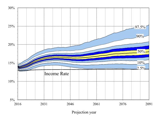
1
For each simulation, the stochastic method develops year-by-year random variation for each variable using Monte Carlo techniques. Each simulation produces an estimate of the financial status of the combined OASI and DI Trust Funds. This appendix shows the distribution of results from 5,000 simulations of the model.
Readers should interpret the results from this model with caution and with an understanding of the model’s limitations. Results are sensitive to equation specifications, degrees of interdependence among variables, and the historical periods used for the estimates. For some variables, recent historical variation may not provide a realistic representation of the potential variation for the future. Also, results would differ if additional variables (such as labor force participation rates, retirement rates, marriage rates, and divorce rates) were also allowed to vary randomly. Furthermore, more variability would result if statistical approaches were used to model uncertainty in the central tendencies of the variables. Time-series modeling reflects only what occurred in the historical period. Future uncertainty exists not only for the underlying central tendency but also for the frequency and size of occasional longer-term shifts in the central tendency. Many experts predict, and history suggests, that the future will likely bring substantial shifts that are not fully reflected in the current model. As a result, readers should understand that the true range of uncertainty is larger than indicated in this appendix.
3. Stochastic Results
This section illustrates the results for the stochastic simulations of two fundamental measures of actuarial status: the annual cost rates and the trust fund ratio. The latter measure is highlighted in the Overview of this report. Section 4 follows with a comparison of stochastic results to results from the alternative scenarios for these and other measures, and an analysis of the differences.
Figure VI.E1 displays the probability distribution of the year-by-year OASDI cost rates (that is, cost as a percentage of taxable payroll). The range of the annual cost rates widens as the projections move further into the future, which reflects increasing uncertainty. Because there is relatively little variation in income rates across the 5,000 stochastic simulations, the figure includes the income rate only under the intermediate assumptions. The two extreme lines in this figure illustrate the range within which future annual cost rates are projected by the current model to occur 95 percent of the time (i.e., a 95-percent confidence interval). In other words, the current model indicates that there is a 2.5 percent probability that the cost rate for a given year will exceed the upper end of this range and a 2.5 percent probability that it will fall below the lower end of this range. Other lines in the figure delineate additional confidence intervals (80‑percent, 60‑percent, 40‑percent, and 20‑percent) around future annual cost rates. The median (50th percentile) cost rate for each year is the rate for which half of the simulated outcomes are higher and half are lower for that year. These lines do not represent the results of individual stochastic simulations. Instead, for each given year, they represent the percentile distribution of annual cost rates based on all stochastic simulations for that year.
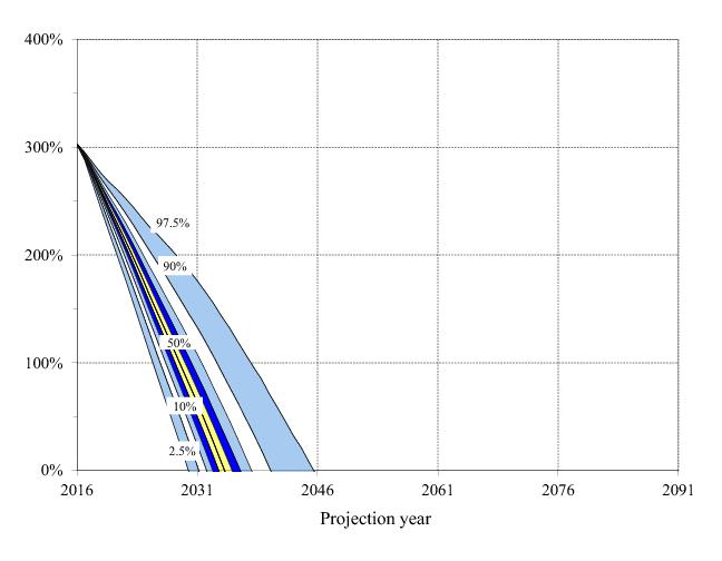
Figure VI.E2 presents the simulated probability distribution of the annual trust fund ratios for the combined OASI and DI Trust Funds. The lines in this figure display the median set (50th percentile) of estimated annual trust fund ratios and delineate the 95‑percent, 80‑percent, 60‑percent, 40‑percent, and 20‑percent confidence intervals expected for future annual trust fund ratios. Again, none of these lines represents the time path of a single simulation. For each given year, they represent the percentile distribution of trust fund ratios based on all stochastic simulations for that year.
Figure VI.E2 shows that the 95‑percent confidence interval for the trust fund depletion year ranges from 2029 to 2045, and there is a 50‑percent probability of trust fund depletion by the end of 2034 (the median depletion year). The median depletion year is the same as the Trustees project under the intermediate assumptions. The figure also shows confidence intervals for the trust fund ratio in each year. For example, the 95‑percent confidence interval for the trust fund ratio in 2025 ranges from 227 to 110 percent of annual cost.
4. Comparison of Results: Stochastic to Low-Cost, Intermediate, and High-Cost Alternatives
This section compares results from two different approaches for illustrating ranges of uncertainty for trust fund actuarial status. One approach uses results from the low-cost, intermediate, and high-cost alternative scenarios. The other approach uses distributions of results from 5,000 independent stochastic simulations. Each of these approaches provides insights into uncertainty. Comparison of the results requires an understanding of fundamental differences in the approaches.
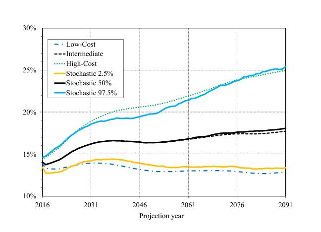
One fundamental difference relates to the presentation of distributional results. Figure VI.E3 shows projected OASDI annual cost rates for the low-cost, intermediate, and high-cost alternatives along with the annual cost rates at the 97.5th percentile, 50th percentile, and 2.5th percentile for the stochastic simulations. While all values on each line for the alternatives are results from a single specified scenario, the values on each stochastic line may be results from different simulations for different years. The one stochastic simulation (from the 5,000 simulations) that yields results closest to a particular percentile for one projected year may yield results that are distant from that percentile in another projected year.
Because each stochastic simulation shows substantial variability from year to year, the range shown between the 97.5th and 2.5th percentiles is broader than would be seen if simulations followed a smooth trend like in the alternatives. In spite of this effect, the range from high-cost to low-cost annual rates for the stochastic distribution is generally contained slightly within the range for the high-cost and low-cost alternatives. With introduction of parameter uncertainty for the stochastic simulations expected in future reports, the range for the 95-percent confidence interval is expected to expand.
Both the alternatives and the stochastic results suggest that the range of potential cost rates above the central levels (those for the intermediate alternative and for the median, respectively) is larger than the range below these central results. The difference between the central results and the higher cost levels (the high-cost alternative and the upper end of the 95-percent confidence range, respectively) is about 1.5 times as large as the difference between the central and lower cost levels for both models by the end of the projection period.
Another fundamental difference between the alternatives and the stochastic simulations is the method of assigning values for assumptions. For the alternatives, specific values are assigned for each of the key demographic and economic variables. Values for all parameters that affect annual cost or payroll are assigned to the high-cost alternative in order to raise estimated annual cost as a percent of payroll, and values are assigned to the low-cost alternative in order to reduce it. (One parameter, the interest rate, has no effect on annual cost as a percent of payroll.) In contrast, the stochastic method essentially randomly assigns values for each of the key demographic and economic variables for each year in each of the 5,000 independent stochastic simulations. For each of the stochastic simulations, randomly assigned values for different variables result in varying and often offsetting effects on projected cost as a percent of payroll, with some tending toward higher cost and some tending toward lower cost. This difference tends to reduce the range of cost as a percent of payroll across the 95-percent confidence interval. Again, the future introduction of parameter uncertainty is expected to broaden this range.
It is important to understand that the stochastic model’s 95-percent confidence intervals for any summary measure of trust fund finances would tend to be narrower than the range produced for the low-cost and high-cost alternatives, even if the stochastic model’s 95-percent confidence interval for annual cost rates were identical to the range defined by the low-cost and high-cost projections. This is true because summary measures of trust fund finances depend on cost rates for many years, and the probability that annual cost rates, on average for individual stochastic simulations, will be at least as low (high) as the 2.5 (97.5) percentile line is significantly lower than 2.5 percent. As a result, the relationship between the ranges presented for annual cost rates and summary measures of trust fund finances is fundamentally different for the stochastic model than it is for the low-cost and high-cost alternatives.
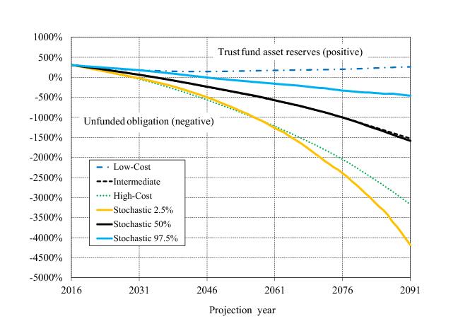
Figure VI.E4 compares the ranges of trust fund (unfunded obligation) ratios for the alternative scenarios and the 95-percent confidence interval of the stochastic simulations. This figure extends figure VI.E2 to show unfunded obligation ratios, expressed as negative values below the zero percent line. An unfunded obligation ratio is the ratio of the unfunded obligation accumulated through the beginning of the year to the cost for that year.
Figure VI.E4.—OASDI Trust Fund (Unfunded Obligation) Ratios: Comparison of Stochastic to Low-Cost, Intermediate, and High-Cost Alternatives1

1
An unfunded obligation, shown as a negative value in this figure, is equivalent to the amount the trust funds would need to have borrowed to date in order to pay all scheduled benefits (on a timely basis) after trust fund asset reserves are depleted. Note that current law does not permit the trust funds to borrow.
 

As mentioned above, a summary measure that accumulates annual values tends to smooth the kind of annual fluctuations that occur in stochastic simulations. Therefore, one might expect the range across the stochastic confidence interval for trust fund (unfunded obligation) ratios to be narrower and fall within the range seen across the high-cost and low-cost alternatives, as it does for the actuarial balance measure. But this is not the case, largely due to the way interest rates are assigned.
For the stochastic model, real interest rates for each simulation are assigned essentially randomly, so the rate for compounding of trust fund reserves (unfunded obligations) is essentially uncorrelated with the level of cost as a percent of payroll. On the other hand, real interest rates are assigned to be higher for the low-cost alternative and lower for the high-cost alternative. High interest rates raise the level of the positive trust fund ratio in the low-cost alternative somewhat, but this effect is limited because the magnitude of reserves is small. However, low interest rates substantially reduce the magnitude of the unfunded obligation ratio for the high-cost alternative because the magnitude of unfunded obligations is relatively large. As a result, the trust fund (unfunded obligation) ratios are shifted, albeit unevenly, higher (or less negative) for both the high-cost and low-cost alternatives.
This interest rate effect on the alternatives is not as evident for some other summary measures of actuarial status, such as the actuarial balance. Because the actuarial balance reflects the cumulative effects of interest in both its numerator and denominator, the interest rate effect is much less pronounced. In contrast, cumulative interest affects only the numerator of the trust fund (unfunded obligation) ratio. There is also no significant interest rate effect on the trust fund depletion date.
Other factors also contribute, to varying degrees, to the difference in ranges between the results of the alternative scenarios and the stochastic simulations. The contrasts in results and methods do not mean that either approach to illustrating ranges of uncertainty is superior to the other. The ranges are different and explainable.
Table VI.E1 displays long-range actuarial estimates for the combined OASDI program using the two methods of illustrating uncertainty: alternative scenarios and stochastic simulations. The table shows stochastic estimates for the median (50th percentile) and for the 95‑percent and 80‑percent confidence intervals. For comparison, the table shows scenario-based estimates for the intermediate, low-cost, and high-cost assumptions. Each individual stochastic estimate in the table is the level at that percentile from the distribution of the 5,000 simulations. For each given percentile, the values in the table for each long-range actuarial measure are generally from different stochastic simulations.
The median stochastic estimates displayed in table VI.E1 are, in general, slightly more pessimistic than the intermediate scenario-based estimates. The median estimate of the long-range actuarial balance is ‑2.67 percent of taxable payroll, about 0.01 percentage point lower than projected under the intermediate assumptions. The median first projected year that cost exceeds non-interest income (as it did in 2010 through 2015), and remains in excess of non-interest income throughout the remainder of the long-range period, is 2016. This is the same year as projected under the intermediate assumptions. The median year that asset reserves first become depleted is 2034, also the same as projected under the intermediate assumptions. The median estimates of the annual cost rate for the 75th year of the projection period are 18.01 percent of taxable payroll and 6.26 percent of gross domestic product (GDP). The comparable estimates under the intermediate assumptions are 17.68 percent of payroll and 6.14 percent of GDP.
For three measures in table VI.E1 (the actuarial balance, the first year cost exceeds non-interest income and remains in excess through 2090, and the first projected year asset reserves become depleted), the 95‑percent stochastic confidence interval is narrower than the range defined by the low-cost and high-cost alternatives. In other words, for these measures, the range defined by the low-cost and high-cost alternatives contains the 95‑percent confidence interval of the stochastic modeling projections. For the remaining three measures (the open group unfunded obligation, the annual cost in the 75th year as a percent of taxable payroll, and the annual cost in the 75th year as a percent of GDP), one or both of the bounds of the 95‑percent stochastic confidence interval fall outside the range defined by the low-cost and high-cost alternatives.
First projected year cost exceeds non-interest income and remains
in excess
through 20901
First year asset reserves become depleted3

1
Cost also exceeded non-interest income in 2010 through 2015.

2
The annual balance is projected to be negative for a temporary period, returning to positive levels before the end of the projection period.

3
For some stochastic simulations, the first year in which trust fund reserves become depleted does not indicate a permanent depletion of reserves.

4
Trust fund reserves are not estimated to be depleted within the projection period.


1
More detail on this model, and stochastic modeling in general, is available at
www.ssa.gov/OACT/stochastic/index.html.


Table of Contents Previous Next Tables Figures Index
SSA Home | Privacy Policy | Website Policies & Other Important Information | Site Map | Actuarial Publications June 22, 2016