2026 OASDI Trustees Report

C. PROGRAM-SPECIFIC ASSUMPTIONS AND METHODS

The Social Security Administration’s Actuarial Services department uses a set of models to project future income and cost under the OASDI program. These models rely not only on the demographic and economic assumptions described in the previous sections, but also on program-specific assumptions and methods. Values of many program parameters change from year to year as prescribed by formulas set out in the Social Security Act. These program parameters affect the level of payroll taxes collected and the level of benefits paid. Actuarial Services uses complex models to project the numbers of future workers covered under OASDI and the levels of their covered earnings, as well as the numbers of future beneficiaries and the expected levels of their benefits. The following subsections provide descriptions of these program-specific assumptions and methods.

1. Automatically Adjusted Program Parameters

The Social Security Act requires that certain parameters affecting the determination of OASDI benefits and taxes be adjusted annually to reflect changes in particular economic measures. Formulas prescribed in the law, applied to reported statistics, change these program parameters annually. The law bases these automatic adjustments on measured changes in the national average wage index (AWI) and the Consumer Price Index for Urban Wage Earners and Clerical Workers (CPI).¹ This section shows values for program parameters adjusted using these indices from the time that these adjustments became effective through 2035. Projected values for future years depend on the economic assumptions described in the preceding section of this report.

Tables V.C1 and V.C2 present the historical and projected values of the CPI-based benefit increases, the AWI series, and the values of many of the wage-indexed program parameters. Each table shows projections under the three alternative sets of assumptions. Table V.C1 includes:

•

The annual cost-of-living benefit increase percentages. The automatic cost-of-living adjustment provisions in the Social Security Act specify increases in OASDI monthly benefits based on increases in the CPI. In general, the benefit increase equals the percentage increase in the CPI measured from the third quarter of the last year with a benefit increase to the third quarter of the current year. If there is no increase in the CPI, there is no benefit increase. All three sets of assumptions include annual cost-of-living adjustments for all future years.

•

The annual levels of and percentage increases in the AWI. Under section 215(b)(3) of the Social Security Act, Social Security benefit computations index taxable earnings (for most workers first becoming eligible for benefits in 1979 or later) using the AWI for each year after 1950. This procedure converts a worker’s past taxable earnings to approximately average-wage-indexed equivalent values near the time of their benefit eligibility. Other program parameters presented in this section that are subject to the automatic-adjustment provisions also rely on the AWI.

•

The wage-indexed contribution and benefit base. For any year, the contribution and benefit base is the maximum amount of covered earnings subject to the OASDI payroll tax and creditable toward benefit computation. The Social Security Act defers any increase in the contribution and benefit base if there is no cost-of-living adjustment effective for December of the preceding year. Under all three sets of assumptions, the contribution and benefit base is projected to increase for all future years.

•

The wage-indexed retirement earnings test exempt amounts. The exempt amounts are the annual amount of earnings below which beneficiaries do not have benefits withheld. A lower exempt amount applies for years prior to the year of attaining normal retirement age. A higher exempt amount applies beginning with the year in which a beneficiary attains normal retirement age. Starting in 2000, the retirement earnings test no longer applies beginning with the month of attaining normal retirement age. The Social Security Act defers any increase in these exempt amounts if there is no cost-of-living adjustment effective for December of the preceding year. Under all three sets of assumptions, the exempt amounts increase for all future years.

Table V.C1.—Cost-of-Living Benefit Increases, Average Wage Index, Contribution and Benefit Bases, and Retirement Earnings Test Exempt Amounts, 1975-2035 

Calendar year		Cost-of-living benefit increasea (percent)	Average wage index (AWI)  b		Contribution and benefit base c	Retirement earnings test exempt amount
			Amount	Increase (percent)		Under NRAd	At NRAe
Historical data:
	1975	8.0	$8,630.92	7.5	$14,100	$2,520	$2,520
	1976	6.4	9,226.48	6.9	15,300	2,760	2,760
	1977	5.9	9,779.44	6.0	16,500	3,000	3,000
	1978	6.5	10,556.03	7.9	17,700	3,240	4,000
	1979	9.9	11,479.46	8.7	22,900	3,480	4,500
	1980	14.3	12,513.46	9.0	25,900	3,720	5,000
	1981	11.2	13,773.10	10.1	29,700	4,080	5,500
	1982	7.4	14,531.34	5.5	32,400	4,440	6,000
	1983	3.5	15,239.24	4.9	35,700	4,920	6,600
	1984	3.5	16,135.07	5.9	37,800	5,160	6,960
	1985	3.1	16,822.51	4.3	39,600	5,400	7,320
	1986	1.3	17,321.82	3.0	42,000	5,760	7,800
	1987	4.2	18,426.51	6.4	43,800	6,000	8,160
	1988	4.0	19,334.04	4.9	45,000	6,120	8,400
	1989	4.7	20,099.55	4.0	48,000	6,480	8,880
	1990	5.4	21,027.98	4.6	51,300	6,840	9,360
	1991	3.7	21,811.60	3.7	53,400	7,080	9,720
	1992	3.0	22,935.42	5.2	55,500	7,440	10,200
	1993	2.6	23,132.67	.9	57,600	7,680	10,560
	1994	2.8	23,753.53	2.7	60,600	8,040	11,160
	1995	2.6	24,705.66	4.0	61,200	8,160	11,280
	1996	2.9	25,913.90	4.9	62,700	8,280	12,500
	1997	2.1	27,426.00	5.8	65,400	8,640	13,500
	1998	1.3	28,861.44	5.2	68,400	9,120	14,500
	1999	f 2.5	30,469.84	5.6	72,600	9,600	15,500
	2000	3.5	32,154.82	5.5	76,200	10,080	17,000
	2001	2.6	32,921.92	2.4	80,400	10,680	25,000
	2002	1.4	33,252.09	1.0	84,900	11,280	30,000
	2003	2.1	34,064.95	2.4	87,000	11,520	30,720
	2004	2.7	35,648.55	4.6	87,900	11,640	31,080
	2005	4.1	36,952.94	3.7	90,000	12,000	31,800
	2006	3.3	38,651.41	4.6	94,200	12,480	33,240
	2007	2.3	40,405.48	4.5	97,500	12,960	34,440
	2008	5.8	41,334.97	2.3	102,000	13,560	36,120
	2009	.0	40,711.61	-1.5	106,800	14,160	37,680
	2010	.0	41,673.83	2.4	106,800	14,160	37,680
	2011	3.6	42,979.61	3.1	106,800	14,160	37,680
	2012	1.7	44,321.67	3.1	110,100	14,640	38,880
	2013	1.5	44,888.16	1.3	113,700	15,120	40,080
	2014	1.7	46,481.52	3.5	117,000	15,480	41,400
	2015	.0	48,098.63	3.5	118,500	15,720	41,880
	2016	.3	48,642.15	1.1	118,500	15,720	41,880
	2017	2.0	50,321.89	3.5	127,200	16,920	44,880
	2018	2.8	52,145.80	3.6	128,400	17,040	45,360
	2019	1.6	54,099.99	3.7	132,900	17,640	46,920
	2020	1.3	55,628.60	2.8	137,700	18,240	48,600
	2021	5.9	60,575.07	8.9	142,800	18,960	50,520
	2022	8.7	63,795.13	5.3	147,000	19,560	51,960
	2023	3.2	66,621.80	4.4	160,200	21,240	56,520
	2024	2.5	69,846.57	4.8	168,600	22,320	59,520
Intermediate:
	2025	g2.8	$72,025.07	3.1	g$176,100	g$23,400	g$62,160
	2026	2.7	75,246.70	4.5	g184,500	g24,480	g65,160
	2027	2.4	78,286.92	4.0	190,200	25,200	67,200
	2028	2.4	81,537.43	4.2	198,900	26,400	70,200
	2029	2.4	85,047.82	4.3	206,700	27,480	73,080
	2030	2.4	88,895.99	4.5	215,400	28,560	76,080
	2031	2.4	92,915.31	4.5	224,700	29,760	79,320
	2032	2.4	96,989.47	4.4	234,900	31,200	82,920
	2033	2.4	101,085.63	4.2	245,400	32,520	86,640
	2034	2.4	105,045.59	3.9	256,200	33,960	90,480
	2035	2.4	109,064.86	3.8	267,000	35,400	94,320
Low-cost:
	2025	g2.8	71,915.14	3.0	g176,100	g23,400	g62,160
	2026	2.9	75,850.68	5.5	g184,500	g24,480	g65,160
	2027	3.0	79,891.38	5.3	189,900	25,200	67,080
	2028	3.0	84,348.74	5.6	200,400	26,640	70,800
	2029	3.0	89,067.21	5.6	211,200	27,960	74,520
	2030	3.0	94,117.03	5.7	222,900	29,520	78,720
	2031	3.0	99,492.97	5.7	235,200	31,200	83,040
	2032	3.0	105,213.03	5.7	248,700	33,000	87,840
	2033	3.0	111,185.04	5.7	262,800	34,920	92,880
	2034	3.0	117,304.17	5.5	278,100	36,840	98,160
	2035	3.0	123,623.86	5.4	293,700	39,000	103,680
High-cost:
	2025	g2.8	72,072.27	3.2	g176,100	g23,400	g62,160
	2026	2.3	74,045.50	2.7	g184,500	g24,480	g65,160
	2027	1.8	74,522.43	.6	190,500	25,320	67,200
	2028	1.8	76,817.19	3.1	195,600	25,920	69,120
	2029	1.8	79,314.73	3.3	196,800	26,160	69,480
	2030	1.8	82,233.65	3.7	203,100	26,880	71,640
	2031	1.8	85,278.60	3.7	209,700	27,840	74,040
	2032	1.8	88,286.58	3.5	217,200	28,800	76,680
	2033	1.8	91,004.77	3.1	225,300	29,880	79,560
	2034	1.8	93,559.46	2.8	233,400	30,960	82,320
	2035	1.8	96,089.74	2.7	240,600	31,920	84,960

---

a

Effective with benefits payable for June in each year 1975-82, and for December in each year after 1982.

b

See table VI.G1 for projected dollar amounts of the AWI for years beyond the last year of this table.

c

Public Law 95-216 specified amounts for 1978-81. Public Law 101-239 changed the indexing procedure and caused slightly higher bases after 1989.

d

Normal retirement age. See table V.C3 for specific values.

e

In 1955-82, the retirement earnings test did not apply at ages 72 and over. In 1983-99, the test did not apply at ages 70 and over. Beginning in 2000, the test does not apply beginning with the month of normal retirement age attainment. In the year of normal retirement age attainment, the higher exempt amount applies to earnings prior to the month of normal retirement age attainment. Public Law 95-216 specified amounts for 1978-82. Public Law 104‑121 specified amounts for 1996-2002.

f

Originally determined as 2.4 percent. Pursuant to Public Law 106-554, effectively 2.5 percent.

g

Actual amount, as determined under automatic-adjustment provisions.

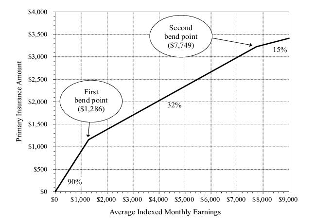
Table V.C2 shows values for other wage-indexed parameters. The table provides historical values from 1978, when indexing of the amount of covered earnings required for a quarter of coverage first began, through 2026, and also shows projected values through 2035. These other wage-indexed program parameters are:

•

The bend points in the formula for computing the primary insurance amount (PIA) for workers who reach age 62, become disabled, or die in a given year. As figure V.C1 illustrates, these two bend points define three ranges in a worker’s average indexed monthly earnings (AIME). The formula for the worker’s PIA multiplies a 90, 32, or 15 percent factor by the portion of the worker’s AIME that falls within the three respective ranges, and then adds the resulting products together.

Figure V.C1.—Primary-Insurance-Amount Formula for Those Newly Eligible in 2026

[D]

•

The bend points in the formula for computing the maximum total amount of monthly benefits payable based on the earnings record of a retired or deceased worker (maximum family benefit). As figure V.C2 illustrates, these three bend points define four ranges in a worker’s PIA. The formula for the maximum family benefit multiplies a 150, 272, 134, or 175 percent factor by the portion of the worker’s PIA that falls within the four respective ranges, and then adds the resulting products together.

Figure V.C2.—OASI Maximum-Family-Benefit Formula
for Those Newly Eligible in 2026

[D]

•	The amount of covered earnings required in a year to earn a quarter of coverage (QC). The number and timing of QCs earned determines an individual’s insured status — the basic requirement for benefit eligibility under OASDI.

•

The old-law contribution and benefit base—the contribution and benefit base that would have been in effect without enactment of the 1977 amendments. This old-law base has four primary uses: (1) it is used in determining special-minimum benefits for certain workers who have many years of low earnings in covered employment; (2) from 1986 through 2023, the calculation of OASDI benefits for certain workers who were eligible to receive pensions based on noncovered employment2 used the old-law base; (3) the Railroad Retirement program uses this base for certain purposes; and (4) the Employee Retirement Income Security Act of 1974 requires the old-law base to be used in various computations and determinations for retirement plans.

Table V.C2.—Values for Selected Wage-Indexed Program Parameters,
Calendar Years 1978-2035 

Calendar year		AIME bend points in PIA formula a			PIA bend points in OASI maximum- family-benefit formula b			Earnings required for a quarter of coverage	Old-law contribution and benefit base c
		First	Second		First	Second	Third
Historical data:
	1978	d	d		d	d	d	e $250	e $17,700
	1979	e $180	e $1,085		e $230	e $332	e $433	260	18,900
	1980	194	1,171		248	358	467	290	20,400
	1981	211	1,274		270	390	508	310	22,200
	1982	230	1,388		294	425	554	340	24,300
	1983	254	1,528		324	468	610	370	26,700
	1984	267	1,612		342	493	643	390	28,200
	1985	280	1,691		358	517	675	410	29,700
	1986	297	1,790		379	548	714	440	31,500
	1987	310	1,866		396	571	745	460	32,700
	1988	319	1,922		407	588	767	470	33,600
	1989	339	2,044		433	626	816	500	35,700
	1990	356	2,145		455	656	856	520	38,100
	1991	370	2,230		473	682	890	540	39,600
	1992	387	2,333		495	714	931	570	41,400
	1993	401	2,420		513	740	966	590	42,900
	1994	422	2,545		539	779	1,016	620	45,000
	1995	426	2,567		544	785	1,024	630	45,300
	1996	437	2,635		559	806	1,052	640	46,500
	1997	455	2,741		581	839	1,094	670	48,600
	1998	477	2,875		609	880	1,147	700	50,700
	1999	505	3,043		645	931	1,214	740	53,700
	2000	531	3,202		679	980	1,278	780	56,700
	2001	561	3,381		717	1,034	1,349	830	59,700
	2002	592	3,567		756	1,092	1,424	870	63,000
	2003	606	3,653		774	1,118	1,458	890	64,500
	2004	612	3,689		782	1,129	1,472	900	65,100
	2005	627	3,779		801	1,156	1,508	920	66,900
	2006	656	3,955		838	1,210	1,578	970	69,900
	2007	680	4,100		869	1,255	1,636	1,000	72,600
	2008	711	4,288		909	1,312	1,711	1,050	75,900
	2009	744	4,483		950	1,372	1,789	1,090	79,200
	2010	761	4,586		972	1,403	1,830	1,120	79,200
	2011	749	4,517		957	1,382	1,803	1,120	79,200
	2012	767	4,624		980	1,415	1,845	1,130	81,900
	2013	791	4,768		1,011	1,459	1,903	1,160	84,300
	2014	816	4,917		1,042	1,505	1,962	1,200	87,000
	2015	826	4,980		1,056	1,524	1,987	1,220	88,200
	2016	856	5,157		1,093	1,578	2,058	1,260	88,200
	2017	885	5,336		1,131	1,633	2,130	1,300	94,500
	2018	895	5,397		1,144	1,651	2,154	1,320	95,400
	2019	926	5,583		1,184	1,708	2,228	1,360	98,700
	2020	960	5,785		1,226	1,770	2,309	1,410	102,300
	2021	996	6,002		1,272	1,837	2,395	1,470	106,200
	2022	1,024	6,172		1,308	1,889	2,463	1,510	109,200
	2023	1,115	6,721		1,425	2,056	2,682	1,640	118,800
	2024	1,174	7,078		1,500	2,166	2,825	1,730	125,100
	2025	1,226	7,391		1,567	2,262	2,950	1,810	130,800
	2026	1,286	7,749		1,643	2,371	3,093	1,890	137,100
Intermediate:
	2027	1,326	7,991		1,694	2,445	3,189	1,950	141,300
	2028	1,385	8,348		1,770	2,555	3,332	2,040	147,600
	2029	1,441	8,686		1,841	2,658	3,466	2,120	153,600
	2030	1,501	9,046		1,918	2,768	3,610	2,210	159,900
	2031	1,565	9,436		2,000	2,887	3,766	2,300	166,800
	2032	1,636	9,863		2,091	3,018	3,936	2,410	174,300
	2033	1,710	10,309		2,185	3,154	4,114	2,520	182,400
	2034	1,785	10,761		2,281	3,293	4,294	2,630	190,200
	2035	1,861	11,215		2,377	3,432	4,476	2,740	198,300
Low-cost:
	2027	1,324	7,979		1,691	2,441	3,184	1,950	141,000
	2028	1,396	8,415		1,784	2,575	3,358	2,060	148,800
	2029	1,470	8,864		1,879	2,712	3,537	2,160	156,600
	2030	1,553	9,358		1,984	2,864	3,735	2,290	165,600
	2031	1,639	9,882		2,095	3,024	3,944	2,410	174,900
	2032	1,732	10,442		2,214	3,195	4,167	2,550	184,800
	2033	1,831	11,038		2,340	3,378	4,405	2,700	195,300
	2034	1,937	11,673		2,474	3,572	4,658	2,850	206,400
	2035	2,046	12,336		2,615	3,775	4,923	3,010	218,100
High-cost:
	2027	1,327	7,996		1,695	2,447	3,191	1,950	141,300
	2028	1,363	8,215		1,741	2,514	3,278	2,010	145,200
	2029	1,372	8,268		1,753	2,530	3,300	2,020	146,100
	2030	1,414	8,523		1,807	2,608	3,401	2,080	150,600
	2031	1,460	8,800		1,865	2,693	3,512	2,150	155,700
	2032	1,514	9,124		1,934	2,792	3,641	2,230	161,400
	2033	1,570	9,461		2,006	2,895	3,776	2,310	167,400
	2034	1,625	9,795		2,076	2,997	3,909	2,390	173,100
	2035	1,675	10,097		2,140	3,089	4,029	2,470	178,500

---

a

The formula to compute a PIA is: (1) 90% of AIME below the first bend point, plus (2) 32% of AIME in excess of the first bend point but not in excess of the second, plus (3) 15% of AIME in excess of the second bend point. The bend points are determined based on the first year a beneficiary becomes eligible for benefits.

b

The formula to compute an OASI family maximum is: (1) 150% of PIA below the first bend point, plus (2) 272% of PIA in excess of the first bend point but not in excess of the second, plus (3) 134% of PIA in excess of the second bend point but not in excess of the third, plus (4) 175% of PIA in excess of the third bend point. This formula also determines family maximums for disabled-worker beneficiaries first eligible after 1978 and entitled before July 1980.

c

Contribution and benefit base that would have been in effect without enactment of the Social Security Amendments of 1977. Public Law 101-239 changed the indexing procedure and caused slightly higher bases after 1989.

d

No provision in law for this amount in this year.

e

Amount specified by the Social Security Amendments of 1977.

In addition to the economic factors that affect the determination of OASDI benefits, there are certain legislated changes that affect current and future benefit amounts. Two such changes are the scheduled increases in the normal retirement age and in the delayed retirement credits. Table V.C3 shows the scheduled changes in these parameters and the resulting effects on benefit levels expressed as a percentage of PIA.

Table V.C3.—Legislated Changes in Normal Retirement Age and Delayed Retirement
Credits for Persons Attaining Age 62 in Each Year 1986 and Later

Year of birth	Year of attainment of age 62	Normal retirement age (NRA)	Credit for each year of delayed retirement after NRA (percent)	Benefit, as a percentage of PIA, beginning at age —
				62	65	66	67	70
1924	1986	65	3	80	100	103	106	115
1925	1987	65	3 1/2	80	100	103 1/2	107	117 1/2
1926	1988	65	3 1/2	80	100	103 1/2	107	117 1/2
1927	1989	65	4	80	100	104	108	120
1928	1990	65	4	80	100	104	108	120
1929	1991	65	4 1/2	80	100	104 1/2	109	122 1/2
1930	1992	65	4 1/2	80	100	104 1/2	109	122 1/2
1931	1993	65	5	80	100	105	110	125
1932	1994	65	5	80	100	105	110	125
1933	1995	65	5 1/2	80	100	105 1/2	111	127 1/2
1934	1996	65	5 1/2	80	100	105 1/2	111	127 1/2
1935	1997	65	6	80	100	106	112	130
1936	1998	65	6	80	100	106	112	130
1937	1999	65	6 1/2	80	100	106 1/2	113	132 1/2
1938	2000	65, 2 mo	6 1/2	79 1/6	98 8/9	105 5/12	111 11/12	131 5/12
1939	2001	65, 4 mo	7	78 1/3	97 7/9	104 2/3	111 2/3	132 2/3
1940	2002	65, 6 mo	7	77 1/2	96 2/3	103 1/2	110 1/2	131 1/2
1941	2003	65, 8 mo	7 1/2	76 2/3	95 5/9	102 1/2	110	132 1/2
1942	2004	65, 10 mo	7 1/2	75 5/6	94 4/9	101 1/4	108 3/4	131 1/4
1943-54	2005-16	66	8	75	93 1/3	100	108	132
1955	2017	66, 2 mo	8	74 1/6	92 2/9	98 8/9	106 2/3	130 2/3
1956	2018	66, 4 mo	8	73 1/3	91 1/9	97 7/9	105 1/3	129 1/3
1957	2019	66, 6 mo	8	72 1/2	90	96 2/3	104	128
1958	2020	66, 8 mo	8	71 2/3	88 8/9	95 5/9	102 2/3	126 2/3
1959	2021	66, 10 mo	8	70 5/6	87 7/9	94 4/9	101 1/3	125 1/3
1960 & later	2022 & later	67	8	70	86 2/3	93 1/3	100	124

2. Covered Employment

Projections of the total U.S. civilian labor force and unemployment rate (see table V.B2) are based on Bureau of Labor Statistics definitions from the Current Population Survey (CPS). These projections represent the average weekly number of employed and unemployed persons, age 16 and over, in the U.S. in a calendar year. Covered employment for a calendar year is defined as the total number of persons who have any OASDI covered earnings (that is, earnings subject to the OASDI payroll tax) at any time during that year. For those age 16 and over, covered employment is projected as the sum over age-sex groups, each reflecting the growth projected for the group’s total U.S. employment and average weeks worked per year.³ The method of projecting covered employment also accounts for changes in non-OASDI-covered employment, including changes in the number and employment status of temporary or unlawfully present immigrants included in the Social Security area population, as well as the increase in coverage of Federal civilian employment as a result of the 1983 Social Security Amendments.

The covered-worker rate is the ratio of OASDI covered workers to the Social Security area population. For men and boys age 16 and over, the projected age-adjusted covered-worker rates⁴ for 2100 are 68.6, 67.9, and 67.6 percent for the low-cost, intermediate, and high-cost assumptions, respectively. For women and girls age 16 and over, the projected age-adjusted covered-worker rates for 2100 are 65.9, 65.2, and 64.9 percent for the low-cost, intermediate, and high-cost assumptions, respectively. For men and boys, the intermediate projected rate for 2100 is lower than the age-adjusted rate of 68.7 percent for 2024 (the last complete historical year) primarily due to the projected increase in the portion of the Social Security area population that consists of temporary or unlawfully present immigrants. For women and girls, the intermediate projected rate for 2100 is higher than the 2024 age-adjusted rate of 64.0 percent because the projected increase in the age-adjusted labor force participation rate more than offsets the projected increase in the portion of the population that will be temporary or unlawfully present immigrants.

3. Insured Population

Eligibility for worker benefits under the OASDI program requires some threshold level of work in covered employment. A worker satisfies this requirement by their accumulation of quarters of coverage (QCs). Prior to 1978, a worker earned one QC for each calendar quarter in which they had covered earnings of at least $50. In 1978, when annual earnings reporting replaced quarterly reporting, the amount required to earn a QC (up to a maximum of four per year) was set at $250. As specified in the law, the Social Security Administration has adjusted this amount each year since then according to changes in the AWI. Its value in 2026 is $1,890.

There are three types of insured status that a worker can earn under the OASDI program. The number and recency of QCs earned determine each status.

•	A worker is fully insured when their total number of QCs is greater than or equal to the number of years elapsed after the year of attainment of age 21 (but not less than six). After a worker has accumulated 40 QCs, they remain permanently fully insured.

•

A worker is disability insured in a quarter if they are: (1) a fully insured worker who has accumulated 20 QCs during the 40-quarter period ending with the quarter, (2) a fully insured worker aged 24-30 who has accumulated QCs during one-half of the quarters elapsed after the quarter of attainment of age 21 and up to and including the quarter, or (3) a fully insured worker under age 24 who has accumulated six QCs during the 12-quarter period ending with the quarter.

•	A worker is currently insured in a quarter when they have accumulated six QCs during the 13-quarter period ending with the quarter.

Periods of disability can potentially change the period considered and the number of QCs needed for each type of insured status, by excluding quarters within the period of disability from consideration.

There are many types of benefits payable to workers and their family members under the OASDI program. Workers must be fully insured to be eligible for a primary retirement benefit and for their spouses or children to be eligible for auxiliary retirement benefits. Deceased workers must have been either currently insured or fully insured at the time of death for their children (and the children’s mother or father) to be eligible for benefits. If there are no eligible surviving children, deceased workers must have been fully insured at the time of death for their qualifying surviving spouses to be eligible. Workers must be disability insured to be eligible for a primary disability benefit and for their spouses or children to be eligible for auxiliary disability benefits.

Actuarial Services estimates the fully insured population, as a percentage of the Social Security area population, by single year of age and sex starting in 1969. The short-range model extrapolates the historical trend in these rates from data in the Continuous Work History Sample (CWHS). The model uses information on quarters of coverage earned due to employment covered by Social Security derived from tabulations of the CWHS. The model also uses historical administrative data on beneficiaries in force and estimated historical mortality rates. The model combines this information to estimate the proportion of individuals who were alive and fully insured as of the end of each historical year. Using projected mortality rates and covered workers, the model extrapolates these rates into the future and applies them to the historical and projected population to arrive at the fully insured population by age and sex through the end of the short-range period.

The long-range fully insured model uses 30,000 simulated work histories for each sex and birth cohort, representing everyone except the temporary or unlawfully present immigrant population.⁵ For the temporary or unlawfully present immigrant population, the model generates substantially lower percentages attaining fully insured status. The model constructs simulated work histories using past coverage rates, earnings distributions, and amounts required for crediting QCs, and develops them in a manner that replicates historical individual variations in work patterns. The probability of covered employment in any year is assumed to be higher for those who have worked more consistently in the recent past. Model parameters are selected so that simulated fully insured percentages are consistent with the fully insured percentages estimated by the short-range model for the recent historical period.

Actuarial Services estimates the disability insured population, as a percentage of the fully insured population, by age and sex starting in 1969. Historical values are based on a tabulation of the disability insured population from the CWHS and estimates of the fully insured population. The short-range model projects these percentages by using the relationship between the historical percentages and covered-worker rates. The long-range model projects these percentages by using the same simulated work histories used to project the fully insured percentages. The long-range model makes additional adjustments to the model simulations in order to bring the disability insured percentages in the historical and short-range periods into close agreement with those estimated from the CWHS and the short-range model.

The currently insured population is not projected because the number of beneficiaries who are entitled to benefits based solely on currently insured status has been very small recently and is likely to remain small in the future.

Using these insured models, the percentage of the Social Security area population age 62 that is fully insured is projected to change from an estimated level of 90.5 at the end of calendar year 2025 to 87.3, 88.0, and 89.9 at the end of 2100 under the low-cost, intermediate, and high-cost alternatives, respectively. Over the projection period, the percentages for both men and women change significantly. The percentage for men declines, reflecting increases in the percent of the population that is classified as temporary or unlawfully present immigrants and is thus less likely to have earnings reported and credited to them. The percentage for women declines more gradually than the percentage for men. For women, the decrease in the percentage due to increases in temporary or unlawfully present immigrants is partially offset by an increase due to the substantial growth in the employment of younger cohorts of women in recent decades. Under the intermediate assumptions, for example, the percentage for men decreases from 92.6 at the end of 2025 to 88.4 at the end of 2100, while the percentage for women decreases from 88.5 at the end of 2025 to 87.7 at the end of 2100.

The percentage of the Social Security area population age 50 that is disability insured is projected to change from an estimated level of 75.9 at the end of calendar year 2025 to 76.6, 77.4, and 79.5 at the end of 2100 under the low-cost, intermediate, and high-cost alternatives, respectively. The changes in the disability insured percentages over time are affected by the same factors as the fully insured percentages, but they are also influenced by additional recent work criteria, leading to percentages that do not change significantly over the long-range projection period.

4. Old-Age and Survivors Insurance Beneficiaries

Actuarial Services projects the number of OASI beneficiaries for each type of benefit separately by the sex of the worker on whose covered earnings the benefits are based and by the age of the beneficiary. Actuarial Services uses two separate models in making these projections. The short-range model makes projections during the first 10 years of the projection period, reflecting recent and expected short-term trends. The long-range model makes projections thereafter, reflecting anticipated longer-term trends and projecting the number of beneficiaries by marital status for several types of benefits.

The short-range model develops the number of retired-worker beneficiaries by applying award rates to the aged fully insured population, excluding those already receiving retired-worker, disabled-worker, aged-widow(er), or aged-spouse benefits, and by applying termination rates to the number of retired-worker beneficiaries.

The long-range model projects the number of retired-worker beneficiaries who were not previously converted from disabled-worker beneficiary status as a percentage of the exposed population.⁶ For age 62, the model projects this percentage by using a linear regression based on the historical relationship between this percentage, the employment rate⁷ at age 62, and the number of months from age 62 to normal retirement age. The percentage for ages 70 and over is nearly 100 because delayed retirement credits cannot be earned after age 70. The long-range model projects the percentage for each age 63 through 69 based on historical experience with an adjustment for changes in the portion of the primary insurance amount that is payable at each age of entitlement. The model adjusts these percentages for ages 62 through 69 to reflect changes in the normal retirement age.

The long-range model calculates the number of retired-worker beneficiaries previously converted from disabled-worker beneficiary status using an extension of disabled-worker death rates by age, sex, and duration.

Actuarial Services estimates the number of aged-spouse beneficiaries, excluding those who are also receiving a retired-worker benefit, from the population projected by age and sex. Benefits of aged-spouse beneficiaries depend on the earnings records of their husbands or wives, who are referred to as “earners.” The short-range model projects insured aged-spouse beneficiaries in conjunction with the retired-worker beneficiaries. This model projects uninsured aged-spouse beneficiaries by applying award rates to the aged uninsured male or female population and by applying termination rates to the population already receiving such benefits.

The long-range model estimates aged-spouse beneficiaries separately for those married and divorced. The model projects the number of married aged-spouse beneficiaries, by age and sex, by applying a series of factors to the number of spouses, aged 62 and over, in the population. These factors are the probabilities that the spouse and the earner meet all of the conditions of eligibility — that is, the probabilities that: (1) the earner is 62 or over, (2) the earner is insured, (3) the earner is receiving benefits, (4) the spouse is not receiving a benefit for the care of an entitled child, and (5) the spouse is either not insured or is insured but not receiving retired-worker benefits. To calculate the estimated number of aged-spouse beneficiaries, the model applies a projected prevalence rate to the resulting number of spouses. To reflect the Social Security Fairness Act of 2023, an adjustment is also applied to include additional beneficiaries who were previously ineligible for aged-spouse benefits due to receiving a substantial government pension. Due to the Bipartisan Budget Act of 2015, for those turning age 62 in 2016 and later, deemed filing now applies to all retired workers and spouses even after initial entitlement, regardless of age. Thus, spouses who are insured are no longer eligible to delay their retired-worker benefit while receiving an aged-spouse benefit.⁸

The long-range model estimates the number of divorced aged-spouse beneficiaries, by age and sex, by applying the same factors to the number of divorced persons aged 62 and over in the population, with three differences. First, the model applies a factor to reflect the probability that the earner (former spouse) is still alive. If the former spouse is not alive, the person may be entitled to a divorced widow(er) benefit. Second, the model applies a factor to reflect the probability that the marriage to the former spouse lasted at least 10 years. Third, the model does not apply factor (3) in the previous paragraph because, effective January 1985, a divorced person is generally no longer required to wait for the former spouse to receive benefits.

Actuarial Services bases the projected numbers of children under age 18, and students aged 18 and 19, who are eligible for benefits as children of retired-worker beneficiaries, on the projected number of children in the population. The short-range model develops the number of entitled children by applying award rates to the number of children in the population who have two living parents and by applying termination rates to the number of children already receiving benefits.

The long-range model projects separately the number of entitled children by sex of the earner parent. For each age under 18, the model multiplies the projected number of children with a parent aged 62 and over by the ratio of the number of retired workers aged 62 to 71 to the number of members of the population aged 62 to 71. For student beneficiaries, the model multiplies the number of children aged 18 and 19 in the population by the probabilities that: (1) the parent is alive, aged 62 or over, insured, and receiving a retired-worker benefit; and (2) the child is attending high school.

Actuarial Services projects the number of disabled children, aged 18 and over, of retired-worker beneficiaries from the adult population. The short-range model applies award rates to the population and applies termination rates to the number of disabled children already receiving benefits. The long-range model projects the number of disabled children in a manner similar to that used for student children except for an additional factor that reflects the probability of being disabled before age 22.

The short-range model develops the number of spouses of retired workers, who are entitled to spouse benefits because they are caring for a child who is under age 16 or disabled, by applying award rates to the number of awards to children of retired workers and by applying termination rates to the number of young spouses with a child in their care who are already receiving benefits. The long-range model projects the number of young-spouse beneficiaries with a child in their care as a proportion of the number of child beneficiaries of retired workers, including projected changes in average family size.

Actuarial Services projects the number of aged-widow(er) beneficiaries, excluding those who are also receiving a retired-worker benefit, from the population by age and sex. The short-range model projects fully insured aged-widow(er) beneficiaries in conjunction with the retired-worker beneficiaries. The model projects the number of uninsured aged-widow(er) beneficiaries by applying award rates to the aged uninsured male or female population and by applying termination rates to the population already receiving such benefits. The long-range model projects uninsured aged-widow(er) beneficiaries by marital status. The model multiplies the number of widow(er)s in the population aged 60 and over by the probabilities that: (1) the deceased earner is fully insured at death, (2) the widow(er) is not receiving a benefit for the care of an entitled child, and (3) the widow(er) is not fully insured.

To reflect the Social Security Fairness Act of 2023, an adjustment is also applied to include additional beneficiaries who were previously ineligible for aged widow(er) benefits due to receiving a substantial government pension. In addition, the model applies the same factors to the number of divorced persons aged 60 and over in the population and includes additional factors representing the probability that the person’s former earner spouse has died and that the marriage lasted at least 10 years. The model projects the number of insured aged-widow(er) beneficiaries who are ages 60 through 70 in a manner similar to that for uninsured aged-widow(er) beneficiaries. In addition, the model assumes that some insured widow(er)s who had not applied for their retired-worker benefits will receive widow(er) benefits. The model projects insured aged-widow(er) beneficiaries over age 70 by applying termination rates to the population that started receiving such benefits prior to age 70.

The short-range model develops the number of disabled-widow(er) beneficiaries by applying award rates to the male or female population and by applying termination rates to the population already receiving a disabled-widow(er) benefit. The long-range model projects the number for each cohort by age from 50 to normal retirement age as percentages of the widowed and divorced populations, adjusted for the insured status of the deceased spouse, the prevalence of disability, and the probability that the disabled spouse is not receiving another type of benefit.

Actuarial Services bases the projected number of children under age 18, and students aged 18 and 19, who are entitled to benefits as survivors of deceased workers, on the number of children in the population whose mothers or fathers are deceased. The short-range model develops the number of entitled children by applying award rates to the number of orphaned children and by applying termination rates to the number of children already receiving benefits.

The long-range model projects the number of surviving-child beneficiaries in a manner similar to that for student beneficiaries of retired workers, except that the model replaces the probability that the parent is aged 62 or over with the probability that the parent is deceased.

Actuarial Services projects the number of surviving-disabled-child beneficiaries, aged 18 and over, from the adult population. The short-range model applies award rates to the population and applies termination rates to the number of surviving-disabled-child beneficiaries already receiving benefits. The long-range model projects the number of surviving-disabled-child beneficiaries in a manner similar to that for surviving-student-child beneficiaries, except for including an additional factor to reflect the probability of being disabled before age 22.

The short-range model develops the numbers of entitled surviving-mother and surviving-father beneficiaries by applying award rates to the number of awards to surviving-child beneficiaries, in cases where the children are either under age 16 or disabled, and by applying termination rates to the number of surviving-mother and surviving-father beneficiaries already receiving benefits. The long-range model estimates the numbers of surviving-mother and surviving-father beneficiaries, assuming they are not remarried, from the number of surviving-child beneficiaries.

Actuarial Services projects the number of surviving-parent beneficiaries based on the historical pattern of the number of such beneficiaries.

Table V.C4 shows the projected number of beneficiaries under the OASI program by type of benefit. The retired-worker beneficiary counts include those persons who receive a residual auxiliary benefit in addition to their retired-worker benefit. Actuarial Services makes estimates of the number and amount of residual payments separately for spouses and widow(er)s.

Table V.C4.—OASI Beneficiaries With Benefits in Current-Payment Status
at the End of Calendar Years 1945-2100 

[In thousands]

Calendar year		Retired workers and auxiliaries				Survivors				Total
		Workera	Spouse	Child		Widow- widower	Mother- father	Child	Parent
Historical data:
	1945	518	159	13		94	121	377	6	1,288
	1950	1,771	508	46		314	169	653	15	3,477
	1955	4,474	1,192	122		701	292	1,154	25	7,961
	1960	8,061	2,269	268		1,544	401	1,577	36	14,157
	1965	11,101	2,614	461		2,371	472	2,074	35	19,128
	1970	13,349	2,668	546		3,227	523	2,688	29	23,030
	1975	16,589	2,867	643		3,888	582	2,919	21	27,509
	1980	19,564	3,018	639		4,415	563	2,610	15	30,823
	1985	22,435	3,069	456		4,862	372	1,918	10	33,122
	1990	24,841	3,104	421		5,098	304	1,777	6	35,551
	1995	26,679	3,027	441		5,213	275	1,884	4	37,522
	2000	28,505	2,798	459		4,901	203	1,878	3	38,747
	2005	30,461	2,524	488		4,569	178	1,903	2	40,126
	2010	34,593	2,316	580		4,285	159	1,913	2	43,847
	2015	40,089	2,335	648		4,050	140	1,893	1	49,155
	2016	41,233	2,370	661		4,004	133	1,893	1	50,296
	2017	42,447	2,375	675		3,961	128	1,904	1	51,491
	2018	43,721	2,391	690		3,908	121	1,911	1	52,743
	2019	45,094	2,430	701		3,878	117	1,916	1	54,137
	2020	46,330	2,323	704		3,823	115	1,936	1	55,231
	2021	47,293	2,165	687		3,773	114	1,976	1	56,009
	2022	48,588	2,022	682		3,728	112	2,020	1	57,152
	2023	50,148	1,895	685		3,688	108	2,037	1	58,562
	2024	51,773	1,861	713		3,630	104	2,051	1	60,132
	2025	53,625	2,081	734		3,711	99	2,036	1	62,286
Intermediate:
	2026	55,194	2,060	752		3,687	95	2,033	1	63,822
	2030	60,694	1,988	831		3,591	84	2,048	1	69,237
	2035	64,804	1,933	896		3,533	78	2,029	1	73,274
	2040	67,114	1,727	948		3,262	88	2,050	1	75,189
	2045	68,461	1,508	1,023		3,010	98	2,104	1	76,206
	2050	69,911	1,471	1,090		2,854	97	2,097	1	77,519
	2055	72,228	1,474	1,143		2,727	94	2,065	1	79,732
	2060	75,393	1,485	1,196		2,629	89	1,998	1	82,790
	2065	78,350	1,494	1,212		2,579	84	1,912	1	85,632
	2070	81,397	1,494	1,223		2,555	80	1,840	1	88,590
	2075	84,322	1,482	1,230		2,536	77	1,792	1	91,439
	2080	86,339	1,468	1,226		2,493	75	1,760	1	93,362
	2085	87,451	1,453	1,225		2,435	73	1,728	1	94,365
	2090	87,446	1,449	1,213		2,365	70	1,688	1	94,231
	2095	87,135	1,464	1,208		2,303	67	1,641	1	93,819
	2100	87,133	1,488	1,209		2,252	64	1,594	1	93,741
Low-cost:
	2026	55,183	2,061	753		3,688	95	2,035	1	63,814
	2030	60,565	1,994	835		3,589	85	2,064	1	69,133
	2035	64,324	1,950	916		3,521	82	2,100	1	72,893
	2040	65,754	1,704	995		3,299	89	2,259	1	74,102
	2045	66,369	1,472	1,109		3,072	103	2,489	1	74,614
	2050	67,145	1,420	1,211		2,936	104	2,614	1	75,432
	2055	68,808	1,412	1,295		2,826	105	2,675	1	77,122
	2060	71,354	1,404	1,387		2,735	103	2,667	1	79,651
	2065	73,730	1,385	1,433		2,683	102	2,641	1	81,974
	2070	76,142	1,357	1,471		2,652	103	2,650	1	84,374
	2075	78,377	1,323	1,510		2,620	105	2,713	1	86,649
	2080	79,718	1,292	1,535		2,570	109	2,807	1	88,032
	2085	80,207	1,267	1,566		2,509	112	2,888	1	88,550
	2090	79,737	1,264	1,573		2,461	114	2,937	1	88,087
	2095	79,778	1,289	1,601		2,458	115	2,964	1	88,205
	2100	81,492	1,334	1,663		2,487	116	2,994	1	90,085
High-cost:
	2026	55,210	2,059	752		3,687	95	2,032	1	63,835
	2030	60,877	1,984	830		3,596	84	2,034	1	69,406
	2035	65,474	1,920	885		3,555	75	1,964	1	73,874
	2040	69,006	1,757	909		3,195	83	1,825	1	76,777
	2045	71,498	1,553	948		2,908	87	1,730	1	78,725
	2050	74,064	1,538	982		2,723	80	1,618	1	81,004
	2055	77,386	1,569	1,004		2,575	74	1,526	1	84,134
	2060	81,431	1,613	1,018		2,462	67	1,427	1	88,018
	2065	85,150	1,653	1,002		2,407	59	1,323	1	91,594
	2070	88,960	1,677	983		2,376	52	1,228	1	95,277
	2075	92,608	1,687	959		2,359	47	1,146	1	98,806
	2080	95,280	1,683	930		2,315	42	1,076	1	101,326
	2085	96,941	1,666	901		2,251	38	1,013	1	102,811
	2090	97,245	1,649	872		2,160	34	956	1	102,916
	2095	96,372	1,618	844		2,044	31	901	1	101,811
	2100	94,311	1,595	810		1,936	27	848	1	99,528

---

a

Retired-worker beneficiaries include persons who also receive a residual benefit consisting of the excess of an auxiliary benefit over their retired-worker benefit.

Notes:
1. The number of beneficiaries does not include uninsured individuals who receive benefits under section 228 of the Social Security Act. Transfers from the General Fund of the Treasury reimburse the OASI Trust Fund for the cost of most of these individuals.

2. Components may not sum to totals because of rounding.

5. Disability Insurance Beneficiaries

The DI Trust Fund pays for benefits to workers who: (1) satisfy the disability insured requirements, (2) have applied for disabled-worker benefits, (3) are determined to be unable to engage in any substantial gainful activity due to a medically determinable physical or mental impairment severe enough to satisfy the requirements of the program, and (4) have not yet attained normal retirement age. Spouses and children of such disabled-worker beneficiaries may also receive DI benefits provided they satisfy certain criteria, primarily age and earnings requirements.

Actuarial Services projects the number of disabled-worker beneficiaries in current-payment status (disabled-worker prevalence) for each future year. The projections start with the number in current-payment status as of December 2025. Projections of the number of applicants and new beneficiaries awarded benefits each year (disabled-worker incidence) and the number of beneficiaries leaving the disability rolls each year then determine the number in current-payment status in later years. Beneficiaries leave the rolls due to death and recovery (disabled-worker terminations) and due to conversion from disabled-worker to retired-worker beneficiary status at normal retirement age, after which the OASI Trust Fund pays for benefits. The remainder of this section describes the concepts of disabled-worker incidence, termination, and prevalence.

a. Disabled-Worker Incidence

The disabled-worker incidence rate is the ratio of the number of applicants newly awarded disabled-worker benefits during each year to the number of individuals who meet insured requirements but are not yet receiving benefits (the disability-exposed population⁹). Actuarial Services projects the number of newly awarded beneficiaries for each future year by multiplying assumed age-sex-specific disabled-worker incidence rates and the projected disability-exposed population by age and sex.

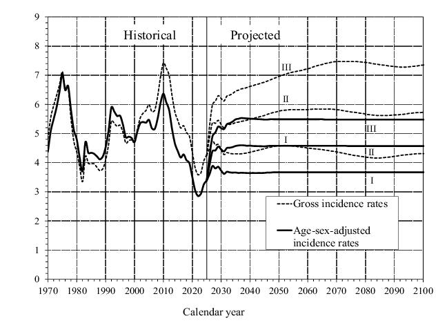
Figure V.C3 illustrates the projected incidence rates under the three alternatives along with historical rates. Incidence rates have varied substantially during the historical period since 1970 due to a variety of demographic and economic factors, along with changes in legislation and program administration. The solid lines in figure V.C3 show the age-sex-adjusted incidence rate consistent with the age-sex distribution of the disability-exposed population for 2000. This adjustment allows a meaningful comparison of incidence rates over time by focusing on the likelihood of being awarded disabled-worker benefits, excluding the effects of a changing distribution of the population toward ages where disability is more or less likely.

The dashed lines in figure V.C3 represent the gross (unadjusted) incidence rates. The changing age‑sex distribution of the exposed population over time influences these unadjusted rates. The gross incidence rate declined relative to the age‑sex-adjusted rate between 1970 and 1990 as the baby-boom generation increased the size of the younger working-age population, where disabled-worker incidence is lower than in older populations. Between 1990 and 2010, the gross rate increased relative to the age‑sex-adjusted rate as the baby-boom generation moved into an age range where disabled-worker incidence is higher. The projected gross incidence rate generally declines relative to the age-sex-adjusted rate as the baby-boom generation moves above the normal retirement age and the lower-birth-rate cohorts of the 1970s enter prime disability ages (50 to normal retirement age). As these smaller cohorts age beyond normal retirement age, by about 2050, the gross incidence rate returns to a higher relative level under the intermediate assumptions. Thereafter, the gross rate remains higher than the age-sex-adjusted rate, reflecting the persistently higher average age of the working-age population compared to the population in 2000, which is largely due to lower birth rates since 1965 and to the increase in the normal retirement age.

For the first 10 years of the projection period (through 2035), incidence rates reflect several factors following on the experience since the recession of 2007-09. At the beginning of the period of high unemployment that began in 2007, disabled-worker incidence rates started to rise to a level well above the general trend level, with rates reaching a peak in 2010. Between 2010 and 2012, incidence rates subsided as the economy recovered, but the decline continued after 2012, reaching levels well below those expected over the long-term. A portion of the elevation of disabled-worker incidence rates experienced during the recession of 2007-09 likely contributed to the lowering of incidence rates experienced during and after the economic recovery that followed, as many individuals applied for disability benefits earlier than they would have otherwise.

For 2025, the actual age-sex-adjusted incidence rate (3.4 per thousand) was well below the level projected in last year’s report (4.4 per thousand). In this year’s report, incidence rates under the intermediate alternative are projected to rise more slowly early in the projection period than in last year’s report, consistent with the low incidence levels experienced recently. Incidence rates are projected to rise to a temporary peak level for 2029, as some of the reduced levels of new benefit awards in recent years are realized in the next few years. The temporary peak in this year’s report is somewhat lower than in last year’s report, consistent with the Social Security Administration’s recent improvements in reducing the time to process disability claims. After 2029, incidence rates decline from the peak, reaching the ultimate assumed level of incidence by the end of the short-range period.

In 2035, at the end of the short-range period, age-sex-specific incidence rates are assumed to reach the ultimate rates assumed for the long-range projections. These ultimate age-sex-specific disabled-worker incidence rates were selected based on careful analysis of historical levels and patterns and expected future conditions, including the impact of scheduled increases in the normal retirement age.¹⁰ The ultimate incidence rates represent the expected average rates of incidence for the future.

For the intermediate alternative, the Trustees assume that the ultimate age-sex-adjusted incidence rate (adjusted to the disability-exposed population for the year 2000) will be 4.6 awards per thousand exposed, which is the same ultimate rate assumed in last year’s report. Figure V.C3 illustrates that the age-sex-adjusted incidence rate averaged 4.9 per thousand over the historical period 1970 through 2025, but it has dropped substantially below that level since 2013. There are a number of factors contributing to this decline in incidence rates, including continuing increases in educational attainment and shifts in occupational composition toward less physically demanding work. These factors and the rates seen in recent years are not consistent with an assumption of a full rise back to longer-term past historical averages. The Trustees continue to monitor experience and review the disabled-worker incidence rate assumption.

The Trustees assume that the ultimate age-sex-adjusted incidence rates for the low-cost and high-cost alternatives will be 3.7 and 5.5 awards per thousand exposed, or about 20 percent lower and higher, respectively, than the ultimate incidence rate for the intermediate alternative. These ultimate low-cost and high-cost incidence rates are both unchanged from those in last year’s report.

Figure V.C3.—Disabled-Worker Incidence Rates

[Awards per thousand disability-exposed]

[D]

b. Disabled-Worker Termination

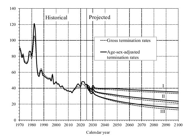
Beneficiaries stop receiving disability benefits when they die, experience an improvement in their medically-determinable impairment such that they are deemed able to engage in substantial gainful activity, or return to substantial work. Disabled-worker beneficiaries who return to substantial work for an extended period are deemed to have recovered, and their benefits are then terminated. The termination rate is the ratio of the number of terminations for these reasons to the average number of disabled-worker beneficiaries during the year.

Actuarial Services projects termination rates by age, sex, and reason for termination. In addition, in the long-range period (post 2035), termination rates are projected by duration of entitlement to disabled-worker benefits.

In the short-range period (through 2035), the projected age-sex-adjusted death termination rate (adjusted to the 2000 disabled-worker beneficiary population) under the intermediate assumptions declines from a rate of 26.3 deaths per thousand beneficiaries for 2025 to about 23.5 per thousand for 2035. The projected age-sex-adjusted recovery rate (medical improvement and return to substantial work) under the intermediate assumptions decreases from the relatively high level of 18.7 per thousand beneficiaries for 2025 to 11.0 per thousand beneficiaries for 2035. The recovery rate has been high in recent years for several reasons, including an ongoing administrative effort to eliminate a backlog of medical continuing disability reviews and to conduct those reviews on a timely basis. The recovery rate is expected to decrease as the backlog of disabled-worker reviews is assumed to be processed over the next several years, with the rate approaching the expected long-term projected rate by 2035. Under the low-cost and high-cost assumptions, total age-sex-adjusted termination rates due to death and recovery are roughly 10 to 20 percent higher and lower, respectively, than under the intermediate assumptions.

For the long-range period (post-2035), Actuarial Services projects death termination and recovery rates by age, sex, and duration of entitlement relative to the average level of rates experienced over the base period 2016 through 2020. Death termination rates by age and sex change throughout the long-range period at the same rate as death rates in the general population. The age-sex-adjusted death termination rate decreases from 26.3 per thousand beneficiaries in 2025 to 21.8, 12.5, and 6.4 per thousand disabled-worker beneficiaries for 2100 under the low-cost, intermediate, and high-cost assumptions, respectively.

The assumed age-sex-adjusted recovery rate for disabled-worker beneficiaries averages 11.1 per thousand beneficiaries for the period 2036 through 2100 under the intermediate alternative, which is 0.3 higher than the average rate assumed in last year’s report. This higher rate reflects the estimated effects of the final rule published on December 31, 2024, establishing an automated wage match with third party payroll data providers. This final rule is expected to increase the number of disability beneficiaries identified with earnings and to identify wages more timely than under prior processes. The assumed age-sex-adjusted recovery rates for the low-cost and high-cost alternatives average 13.3 and 8.9 recoveries per thousand beneficiaries, respectively, for 2036 through 2100. These ultimate low-cost and high-cost recovery rates are similarly higher than in last year’s report by roughly 0.3 per thousand.

Figure V.C4 illustrates gross and age-sex-adjusted total termination rates (including both death terminations and recoveries) for disabled-worker beneficiaries for the historical period since 1970, and for the projection period through 2100. As with incidence rates, the age-sex-adjusted termination rate illustrates the real change in the tendency to terminate benefits. Changes in the age-sex distribution of the beneficiary population influence the gross termination rate. A shift in the disabled-worker beneficiary population to older ages, as occurred over the past 20 years when the baby-boom generation moved into pre-retirement ages, increases gross death termination rates relative to the age-sex-adjusted rates.

Figure V.C4.—Disabled-Worker Termination Rates

[Terminations per thousand disabled-worker beneficiaries]

[D]

c. DI Beneficiaries and Disabled-Worker Prevalence Rates

Incidence and termination rates are the foundation for projecting the number of disabled-worker beneficiaries in current-payment status. At normal retirement age, all disabled-worker beneficiaries automatically convert to retired-worker status and leave the DI rolls.

Actuarial Services makes detailed projections of disabled-worker awards, terminations, and conversions and combines these to project the number of disabled workers receiving benefits over the next 75 years. Table V.C5 presents the projected numbers of disabled-worker beneficiaries in current-payment status. The number of disabled-worker beneficiaries in current-payment status grows from 7.1 million at the end of 2025 to 9.4 million, 10.1 million, and 9.8 million at the end of 2100, under the low-cost, intermediate, and high-cost assumptions, respectively. Much of this increase results from the growth and changing age distribution of the population described earlier in this chapter. Table V.C5 also presents projected numbers of auxiliary beneficiaries and disabled-worker prevalence rates on both a gross basis and an age-sex-adjusted basis.

Table V.C5.—DI Beneficiaries with Benefits in Current-Payment Status
at the End of Calendar Years 1960-2100 

[Beneficiaries in thousands; prevalence rates per thousand insured for disability benefits]

Calendar year		Disabled‑ worker beneficiaries	Auxiliary beneficiaries		Total beneficiaries	Disabled-worker prevalence rates
			Spouse	Child		Gross	Age-sex- adjusteda
Historical data:
	1960	455	77	155	687	9	8
	1965	988	193	558	1,739	18	14
	1970	1,493	283	889	2,665	20	18
	1975	2,488	453	1,411	4,351	29	28
	1980	2,856	462	1,359	4,677	28	31
	1985	2,653	306	945	3,904	24	26
	1990	3,007	266	989	4,261	25	28
	1995	4,179	264	1,409	5,852	33	35
	2000	5,036	165	1,466	6,667	36	36
	2005	6,519	157	1,633	8,309	45	40
	2010	8,204	161	1,820	10,185	55	44
	2015	8,909	143	1,756	10,808	59	45
	2016	8,809	136	1,667	10,612	58	44
	2017	8,695	127	1,590	10,412	56	43
	2018	8,537	119	1,507	10,164	55	41
	2019	8,378	114	1,434	9,927	54	40
	2020	8,151	105	1,364	9,620	52	39
	2021	7,877	97	1,245	9,219	50	36
	2022	7,604	92	1,146	8,842	47	34
	2023	7,366	89	1,061	8,515	45	33
	2024	7,231	87	1,006	8,324	44	32
	2025	7,126	91	949	8,166	43	31
Intermediate:
	2026	7,135	89	923	8,148	43	31
	2030	7,194	83	951	8,228	44	32
	2035	7,475	86	983	8,544	46	34
	2040	8,034	76	1,129	9,239	48	36
	2045	8,790	77	1,307	10,174	51	37
	2050	9,327	82	1,420	10,829	54	38
	2055	9,698	85	1,496	11,279	56	39
	2060	9,778	82	1,517	11,377	57	39
	2065	9,921	82	1,503	11,506	58	40
	2070	9,979	81	1,483	11,543	58	40
	2075	9,837	80	1,474	11,391	58	40
	2080	9,724	79	1,487	11,291	58	40
	2085	9,580	78	1,511	11,170	57	40
	2090	9,661	80	1,534	11,275	57	40
	2095	9,857	83	1,546	11,486	58	41
	2100	10,083	85	1,548	11,717	59	41
Low-cost:
	2026	7,068	89	913	8,070	43	30
	2030	6,691	83	878	7,651	41	30
	2035	6,441	86	868	7,395	39	29
	2040	6,571	61	977	7,610	38	29
	2045	6,996	59	1,165	8,220	39	29
	2050	7,329	61	1,297	8,687	41	29
	2055	7,576	62	1,385	9,023	42	30
	2060	7,635	58	1,416	9,108	41	30
	2065	7,767	57	1,418	9,241	41	30
	2070	7,859	56	1,429	9,344	40	30
	2075	7,840	55	1,470	9,365	40	30
	2080	7,894	55	1,544	9,493	39	30
	2085	8,008	55	1,626	9,688	38	30
	2090	8,408	58	1,696	10,162	39	30
	2095	8,964	62	1,749	10,776	40	31
	2100	9,431	65	1,793	11,288	40	31
High-cost:
	2026	7,203	89	934	8,226	44	31
	2030	7,691	84	1,022	8,797	48	35
	2035	8,495	86	1,086	9,667	53	40
	2040	9,546	91	1,259	10,897	58	43
	2045	10,653	97	1,384	12,134	63	45
	2050	11,398	106	1,442	12,946	68	47
	2055	11,900	112	1,486	13,497	73	49
	2060	11,992	110	1,489	13,592	75	49
	2065	12,126	109	1,455	13,690	78	50
	2070	12,104	109	1,399	13,612	81	50
	2075	11,771	106	1,336	13,213	81	50
	2080	11,390	104	1,281	12,774	82	51
	2085	10,834	99	1,240	12,172	81	51
	2090	10,371	97	1,212	11,681	81	51
	2095	9,942	93	1,185	11,220	81	51
	2100	9,756	94	1,152	11,003	81	51

---

a

Adjusted to the age-sex distribution of the disability insured population for the year 2000.

Note: Components may not sum to totals because of rounding.

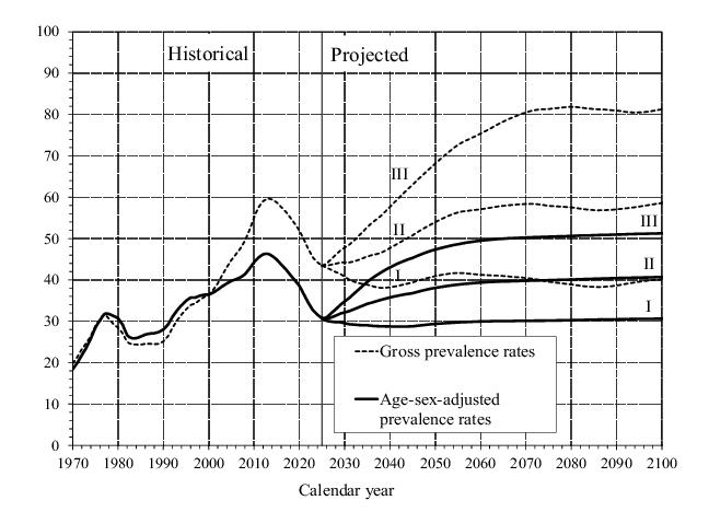
The disabled-worker prevalence rate is the ratio of the number of disabled-worker beneficiaries in current-payment status to the number insured for disability benefits. Figure V.C5 illustrates the historical and projected disabled-worker prevalence rates on both a gross basis and on an age-sex-adjusted basis (adjusted to the age-sex distribution of the disability insured population for the year 2000).

Changes in prevalence rates are a direct result of changes in incidence rates and termination rates. Annual incidence and termination rates are not directly comparable or combinable because their denominators differ.

Figure V.C5.—Disabled-Worker Prevalence Rates
[Rate per thousand insured for disability benefits]

[D]

Age-sex-adjusted prevalence rates increased rapidly from 1990 to about 2013 primarily because: (1) termination rates, in particular death termination rates, declined; (2) incidence rates at younger ages increased relative to rates at older ages (new beneficiaries at younger ages have more potential years on the disability rolls); and (3) incidence rates increased substantially for women to parity with men. Gross prevalence rates increased more than age-sex-adjusted prevalence rates over this period as the baby-boom generation began to reach ages 45 through normal retirement age, ages at which disabled-worker incidence rates are relatively high.

Both age-sex-adjusted and gross prevalence rates have since dropped sharply from the peak in 2013, primarily due to the historically low incidence rates experienced recently. Actuarial Services projects both gross and age-sex-adjusted prevalence rates to begin to grow again in the future, but at a slower pace than between 1990 and 2013, based on assumed stabilization in three factors: (1) the age distribution of the general population, (2) the age distribution of the disability insured population, and (3) incidence rates by age and sex. As these factors gradually stabilize, the declining death termination rate continues to have a small influence toward higher disabled-worker prevalence rates.

As mentioned above in the discussion of incidence and termination rates, the age-sex-adjusted prevalence rate isolates the changing trend in the underlying likelihood of receiving benefits for the insured population, without reflecting changes in the age and sex distribution of the population. As with incidence rates, gross disabled-worker prevalence rates declined relative to the age-sex-adjusted rate when the baby-boom generation reached working age between 1970 and 1990; this trend reflects the lower disabled-worker prevalence rates associated with younger ages. Conversely, the gross rate of disabled-worker prevalence increased relative to the age-sex-adjusted rate from 1990 to 2013 due to the aging of the baby-boom generation into ages with higher disabled-worker prevalence rates.

Under the intermediate assumptions, the projected age-sex-adjusted disabled-worker prevalence rate grows from 30.7 per thousand disability insured workers at the end of 2025 to 40.7 per thousand at the end of 2100. The projected age-sex-adjusted disabled-worker prevalence rate at the end of 2100 is 30.6 per thousand under the low-cost assumptions and 51.3 per thousand under the high-cost assumptions.

Table V.C5 presents projections of the numbers of auxiliary beneficiaries paid from the DI Trust Fund. As indicated at the beginning of this subsection, auxiliary beneficiaries are qualifying spouses and children of disabled-worker beneficiaries. A spouse must either be at least age 62 or have an eligible child beneficiary in their care who is either under age 16 or disabled prior to age 22. A child must be: (1) under age 18, (2) age 18 or 19 and still a student in high school, or (3) age 18 or older and disabled prior to age 22.

The projection of the number of auxiliary beneficiaries relies on the projected number of disabled-worker beneficiaries. In the short-range period (2026 through 2035), Actuarial Services projects incidence and termination rates for each category of auxiliary beneficiary. After 2035, child beneficiaries at ages 18 and under are projected in relation to the projected number of children in the population using the probability that either of their parents is a disabled-worker beneficiary. The remaining categories of children and spouses are projected in a similar manner.

6. Covered and Taxable Earnings, Taxable Payroll, and Payroll Tax Contributions

Covered earnings include covered wages and covered self-employment net earnings. Actuarial Services projects covered wages for component sectors of the economy (i.e., private, State and local government, Federal civilian, and military) based on the projected overall growth of sectoral and total wages in the U.S. economy. The projections of covered wages also reflect changes in covered employment due to a relative increase in non-covered unlawfully present immigrants and to the mandatory coverage of new hires in the Federal civilian sector. Covered self-employment net earnings are projected based on the growth in net proprietors’ income in the U.S. economy.

Taxable earnings are the portion of covered earnings subject to the OASDI payroll tax. Taxable wages for an employee are total covered wages from all wage employment up to the contribution and benefit base. Taxable wages for an employer are the sum of all covered wages paid to each employee up to the base. Employees with multiple jobs whose total wages exceed the base are eligible for a refund of excess employee taxes withheld; employers are not eligible for a refund on this basis. For self-employed workers with no taxable wages, taxable earnings are the amount of covered self-employment net earnings up to the base. For self-employed workers with taxable wages less than the base, covered self-employment net earnings are taxable up to the difference between the base and their taxable wages. For projection purposes, Actuarial Services computes taxable earnings based on a proportion of covered earnings that is at or below the base.

The OASDI taxable payroll (see table VI.G1) for a year is computed as the amount of earnings which, when multiplied by the combined OASDI employee-employer payroll tax rate for that year, yields the total amount of payroll taxes due from wages paid and self-employment net earnings for the year. Taxable payroll is used as the denominator for income rates, cost rates, and actuarial balances. Taxable payroll is derived by adjusting total taxable earnings to account for categories of earnings that are taxed at rates other than the combined employee-employer rate and to take into account amounts credited as wages that were not included in normally reported wages. For 1951 and later, taxable earnings are reduced by one-half of the amount of wages paid to employees with multiple jobs that exceed the contribution and benefit base. For 1983 through 2001, deemed wage credits for military service after 1956 are added to taxable earnings. The self-employment tax rates for 1951 through 1983 were less than the combined employee-employer rates; therefore, the self-employment component of taxable payroll for those years is reduced by multiplying the ratio of the self-employment rate to the combined employee-employer rate times the taxable self-employment net earnings. Finally, for 1966 through 1979, employers were exempt from paying their share of payroll tax on their employees’ tips and, for 1980 through 1987, employers paid tax on only part of their employees’ tips. For those years, the taxable payroll is reduced by half of the amount of tips for which the employer owed no payroll tax.

The ratio of taxable payroll to covered earnings (the taxable ratio) declined from 88.6 percent for 1984 to 82.6 percent for 2000, as earnings for very high earners increased much more than for all other earners. Furthermore, the taxable ratio has usually declined near peaks of economic cycles (such as in 2000) and risen during economic downturns, because earnings for the highest earners often include profit-based incentives and tend to change more with procyclical economic indicators such as corporate profits and stock prices. Specifically, the taxable ratio rose to 85.7 percent for 2002, a year following the 2001 recession; declined to 82.4 percent for 2007, which marked the peak of the economic cycle before the 2007-09 recession; rose to 85.2 percent for 2009, the trough of that recession; and averaged 83.0 percent for the period 2010 to 2019, which encompassed the subsequent recovery and expansion leading to the next economic peak.

During the pandemic-induced recession in 2020, the ratio declined to 82.2 percent from the previous year’s 83.1 percent. Unlike previous economic downturns, this recession led to a greater decrease in earnings for earners at the low end of the earnings distribution than for those at the high end, partly because annual profits and stock prices continued to rise. This resulted in a relatively higher proportion of total wages being above the contribution and benefit base than has typically been the case in other economic downturns. The ratio declined further to 80.4 percent for 2021, as many workers were rehired or newly hired at the low end of the earnings distribution, while some high earners benefited from increased bonuses and the exercising of stock options. As economic growth stabilized closer to the sustainable trend, the taxable ratio increased to 82.0 percent for 2022, to 83.2 percent for 2023, and is estimated to be 82.9 percent for 2024.

For each alternative, the ratio reaches an assumed level at the end of the short-range period (2035). These levels are 84.0 percent for the low-cost assumptions, 82.5 percent for the intermediate assumptions, and 81.0 percent for the high-cost assumptions.¹¹ These are the same assumptions used for the end of the short-range period (2034) in the 2025 report.

Actuarial Services projects payroll tax contributions using the patterns of tax collection required by Federal laws and regulations. Payroll tax liabilities are determined by multiplying the scheduled tax rates for each year by the amount of taxable wages and self-employment net earnings for that year. These liabilities are then split into amounts by collection period. For wages, Federal law requires that employers withhold OASDI and HI payroll taxes and Federal individual income taxes from employees’ pay. As an employer’s accumulation of such taxes (including the employer share of payroll taxes) meets certain thresholds, which the Department of the Treasury determines, the employer must deposit these taxes with the U.S. Treasury by a specific day, depending on the amount of money involved.¹² For projection purposes, payroll tax contributions related to wages are split into amounts paid in the same quarter as incurred and in the following quarter. Self-employed workers must make estimated tax payments on their earnings four times during the year and make up any underestimate on their individual income tax returns. The projected self-employed tax liabilities are split by collection quarter to reflect this pattern.

The projected tax contributions also reflect the method used to ensure that money transferred to the trust funds is adjusted, over time, to equal the actual liability owed. Because payers generally make tax payments without identifying the separate OASDI contribution amounts, Treasury makes daily transfers of money from the General Fund to the trust funds on an initial estimated basis. The Social Security Administration periodically certifies the amounts of wages and self-employment net earnings on which tax contributions are owed for each year, at which time Treasury determines adjustments to appropriations to reconcile tax liabilities with deposits in the trust funds. This process also includes periodic transfers from the trust funds to the General Fund for contributions on wages in excess of the contribution and benefit base.

Table V.C6 shows the payroll tax contribution rates applicable under current law in each calendar year and the allocation of these rates between the OASI and DI Trust Funds.¹³ It also shows the contribution and benefit base for each year through 2026.

Table V.C6.—Contribution and Benefit Base and Payroll Tax Contribution Rates 

Calendar years	Contribution and benefit base	Payroll tax contribution rates (percent)
		Employees and employers, combineda				Self-employedb
		OASDI	OASI	DI		OASDI	OASI	DI
1937-49	$3,000	2.00	2.00	—		—	—	—
1950	3,000	3.00	3.00	—		—	—	—
1951-53	3,600	3.00	3.00	—		2.2500	2.2500	—
1954	3,600	4.00	4.00	—		3.0000	3.0000	—
1955-56	4,200	4.00	4.00	—		3.0000	3.0000	—
1957-58	4,200	4.50	4.00	0.50		3.3750	3.0000	0.3750
1959	4,800	5.00	4.50	.50		3.7500	3.3750	.3750
1960-61	4,800	6.00	5.50	.50		4.5000	4.1250	.3750
1962	4,800	6.25	5.75	.50		4.7000	4.3250	.3750
1963-65	4,800	7.25	6.75	.50		5.4000	5.0250	.3750
1966	6,600	7.70	7.00	.70		5.8000	5.2750	.5250
1967	6,600	7.80	7.10	.70		5.9000	5.3750	.5250
1968	7,800	7.60	6.65	.95		5.8000	5.0875	.7125
1969	7,800	8.40	7.45	.95		6.3000	5.5875	.7125
1970	7,800	8.40	7.30	1.10		6.3000	5.4750	.8250
1971	7,800	9.20	8.10	1.10		6.9000	6.0750	.8250
1972	9,000	9.20	8.10	1.10		6.9000	6.0750	.8250
1973	10,800	9.70	8.60	1.10		7.0000	6.2050	.7950
1974	13,200	9.90	8.75	1.15		7.0000	6.1850	.8150
1975	14,100	9.90	8.75	1.15		7.0000	6.1850	.8150
1976	15,300	9.90	8.75	1.15		7.0000	6.1850	.8150
1977	16,500	9.90	8.75	1.15		7.0000	6.1850	.8150
1978	17,700	10.10	8.55	1.55		7.1000	6.0100	1.0900
1979	22,900	10.16	8.66	1.50		7.0500	6.0100	1.0400
1980	25,900	10.16	9.04	1.12		7.0500	6.2725	.7775
1981	29,700	10.70	9.40	1.30		8.0000	7.0250	.9750
1982	32,400	10.80	9.15	1.65		8.0500	6.8125	1.2375
1983	35,700	10.80	9.55	1.25		8.0500	7.1125	.9375
1984 3	37,800	11.40	10.40	1.00		11.4000	10.4000	1.0000
1985 c	39,600	11.40	10.40	1.00		11.4000	10.4000	1.0000
1986 c	42,000	11.40	10.40	1.00		11.4000	10.4000	1.0000
1987 c	43,800	11.40	10.40	1.00		11.4000	10.4000	1.0000
1988 c	45,000	12.12	11.06	1.06		12.1200	11.0600	1.0600
1989 c	48,000	12.12	11.06	1.06		12.1200	11.0600	1.0600
1990	51,300	12.40	11.20	1.20		12.4000	11.2000	1.2000
1991	53,400	12.40	11.20	1.20		12.4000	11.2000	1.2000
1992	55,500	12.40	11.20	1.20		12.4000	11.2000	1.2000
1993	57,600	12.40	11.20	1.20		12.4000	11.2000	1.2000
1994	60,600	12.40	10.52	1.88		12.4000	10.5200	1.8800
1995	61,200	12.40	10.52	1.88		12.4000	10.5200	1.8800
1996	62,700	12.40	10.52	1.88		12.4000	10.5200	1.8800
1997	65,400	12.40	10.70	1.70		12.4000	10.7000	1.7000
1998	68,400	12.40	10.70	1.70		12.4000	10.7000	1.7000
1999	72,600	12.40	10.70	1.70		12.4000	10.7000	1.7000
2000	76,200	12.40	10.60	1.80		12.4000	10.6000	1.8000
2001	80,400	12.40	10.60	1.80		12.4000	10.6000	1.8000
2002	84,900	12.40	10.60	1.80		12.4000	10.6000	1.8000
2003	87,000	12.40	10.60	1.80		12.4000	10.6000	1.8000
2004	87,900	12.40	10.60	1.80		12.4000	10.6000	1.8000
2005	90,000	12.40	10.60	1.80		12.4000	10.6000	1.8000
2006	94,200	12.40	10.60	1.80		12.4000	10.6000	1.8000
2007	97,500	12.40	10.60	1.80		12.4000	10.6000	1.8000
2008	102,000	12.40	10.60	1.80		12.4000	10.6000	1.8000
2009	106,800	12.40	10.60	1.80		12.4000	10.6000	1.8000
2010d	106,800	12.40	10.60	1.80		12.4000	10.6000	1.8000
2011d	106,800	10.40	8.89	1.51		10.4000	8.8900	1.5100
2012d	110,100	10.40	8.89	1.51		10.4000	8.8900	1.5100
2013	113,700	12.40	10.60	1.80		12.4000	10.6000	1.8000
2014	117,000	12.40	10.60	1.80		12.4000	10.6000	1.8000
2015	118,500	12.40	10.60	1.80		12.4000	10.6000	1.8000
2016	118,500	12.40	10.03	2.37		12.4000	10.0300	2.3700
2017	127,200	12.40	10.03	2.37		12.4000	10.0300	2.3700
2018	128,400	12.40	10.03	2.37		12.4000	10.0300	2.3700
2019	132,900	12.40	10.60	1.80		12.4000	10.6000	1.8000
2020	137,700	12.40	10.60	1.80		12.4000	10.6000	1.8000
2021	142,800	12.40	10.60	1.80		12.4000	10.6000	1.8000
2022	147,000	12.40	10.60	1.80		12.4000	10.6000	1.8000
2023	160,200	12.40	10.60	1.80		12.4000	10.6000	1.8000
2024	168,600	12.40	10.60	1.80		12.4000	10.6000	1.8000
2025	176,100	12.40	10.60	1.80		12.4000	10.6000	1.8000
2026	184,500	12.40	10.60	1.80		12.4000	10.6000	1.8000
2027 and later	e	12.40	10.60	1.80		12.4000	10.6000	1.8000

---

a

Except as noted below, the combined employee/employer rate is divided equally between employees and employers.

b

Beginning in 1990, self-employed persons receive a deduction, for purposes of computing their net earnings, equal to half of the combined OASDI and HI contributions that would be payable without regard to the contribution and benefit base. The OASDI contribution rate then applies to net earnings after this deduction, but subject to the OASDI base.

c

In 1984 only, employees received an immediate credit of 0.3 percent of taxable wages against their OASDI payroll tax contributions. The self-employed received similar credits of 2.7 percent, 2.3 percent, and 2.0 percent against their combined OASDI and Hospital Insurance (HI) contributions on net earnings from self-employment in 1984, 1985, and 1986-89, respectively. The General Fund of the Treasury reimbursed the trust funds for these credits.

d

Public Law 111-147 exempted most employers from paying the employer share of OASDI payroll tax on wages paid during the period March 19, 2010 through December 31, 2010 to certain qualified individuals hired after February 3, 2010. Public Law 111-312 reduced the OASDI payroll tax rate for 2011 by 2 percentage points for employees and for self-employed workers. Public Law 112-96 extended the 2011 rate reduction through 2012. These laws require that the General Fund of the Treasury reimburse the OASI and DI Trust Funds for these temporary reductions in 2010 through 2012 payroll tax revenue, in order to “replicate to the extent possible” revenue that would have been received if the combined employee/employer payroll tax rates had remained at 12.4 percent for OASDI (10.6 percent for OASI and 1.8 percent for DI).

e

Subject to automatic adjustment based on increases in average wages.

7. Income From Taxation of Benefits

Under current law, the OASI and DI Trust Funds are credited with income tax revenue from the taxation of up to the first 50 percent of taxpayers’ OASI and DI benefit payments. (The HI Trust Fund receives the remainder of the income tax revenue from the taxation of up to 85 percent of taxpayers’ OASI and DI benefit payments.) Benefits are partially subject to federal income tax for beneficiaries with income (defined for this purpose as adjusted gross income excluding Social Security benefits, plus half of their Social Security benefits and all of their non-taxable interest income) in excess of specified threshold amounts. The threshold amounts are $25,000 for single filers, $32,000 for joint filers, and $0 for those married individuals filing separately.

For the short-range period, Actuarial Services estimates the income to the OASI and DI Trust Funds from taxation of benefits by applying the following two factors (projected by the Office of Tax Analysis in the Department of the Treasury) to total OASI and DI scheduled benefits: (1) the percentage of taxpayers’ scheduled benefits (limited to 50 percent) that is taxable and (2) the average marginal tax rate applicable to those benefits. Up to 85 percent of benefits may be subject to federal income tax, with any tax on more than 50 percent of a taxpayer’s benefits credited to the Medicare Hospital Insurance Trust Fund.

For the long-range period, Actuarial Services estimates the income to the trust funds from taxation of benefits by applying projected ratios of taxation of OASI and DI benefits to total OASI and DI scheduled benefits. These tax ratios rely on estimates from the Office of Tax Analysis in the Department of the Treasury. Actuarial Services’ estimates reflect the following approach. First, the income thresholds used for benefit taxation are specified in the Internal Revenue Code to be constant in the future, and have never been changed, while income and benefit levels continue to rise. Accordingly, projected ratios of income from taxation of benefits to the amount of benefits increase gradually. Second, because indexation of income tax brackets is not specified in the Social Security Act, and because periodic changes have been made in the past to avoid indefinite compression of the income tax brackets relative to income levels (bracket creep), the Trustees assume that such periodic changes will occur in the future. As a result, after the tenth year of the projection period, income tax brackets are assumed to rise with average wages, rather than with the C-CPI-U as specified under current law. Thus, the income tax brackets are projected to roughly maintain their levels relative to the income distribution.

Note that the One Big Beautiful Bill Act, which the President signed into law on July 4, 2025, made permanent the lower ordinary income tax rates and adjusted tax brackets originally enacted under the Tax Cuts and Jobs Act of 2017. Under the 2017 Act, those brackets were set to expire in 2026. Therefore, Actuarial Services’ estimates no longer incorporate a permanent level shift upward in the ratios for 2026 and beyond.

8. Average Benefits

Projections of average benefits for each benefit type reflect recent historical averages, projected average primary insurance amounts (PIAs), and projected ratios of average benefits to average PIAs. Calculations of average PIAs are based on projected distributions of beneficiaries by duration from year of initial entitlement, average PIAs at initial entitlement, and increases in PIAs after initial entitlement. Projected increases in average PIAs after initial entitlement depend on automatic benefit increases, recomputations to reflect additional covered earnings, and differences in mortality by level of lifetime earnings. Calculations of future average PIAs at initial entitlement are based on projected earnings histories, which in turn reflect a combination of the actual earnings histories associated with a sample of 2022 initial entitlements and more recent actual earnings levels by age and sex for covered workers.

For retired-worker, aged-spouse, and aged-widow(er) benefits, the percentage of the PIA that is payable depends on the age at initial entitlement to benefits. Projected ratios of average benefits to average PIAs for these types of benefits are based on projections of age distributions at initial entitlement.

9. Scheduled Benefits

For each type of benefit, scheduled benefits are the product of the number of beneficiaries and the corresponding average monthly benefit. The short-range model calculates scheduled benefits on a quarterly basis. The long-range model calculates all scheduled benefits on an annual basis, using the number of beneficiaries at the beginning and end of the year. Adjustments to these annual scheduled benefits include retroactive payments to newly awarded beneficiaries and other amounts not reflected in the regular monthly scheduled benefits.

Scheduled lump-sum death benefits are estimated as the product of: (1) the number of lump-sum death payments projected on the basis of the assumed death rates, the projected fully insured population, and the estimated percentage of the fully insured population that will qualify for lump-sum death payments; and (2) the amount of the lump-sum death payment, which is $255 (unindexed since 1973).

10. Illustrative Scheduled Benefit Amounts

Table V.C7 shows, under the intermediate assumptions, future scheduled benefit amounts payable upon retirement at the normal retirement age and at age 65, for various hypothetical workers attaining age 65 in 2026 and subsequent years. The illustrative benefit amounts in table V.C7 are presented in CPI-indexed 2026 dollars—that is, adjusted to 2026 levels by the CPI indexing series shown in table VI.G1. Table V.C7 also shows each benefit amount as a percentage of the average of each hypothetical worker’s highest 35 years of Social Security covered earnings, indexed by national average wage growth to the year prior to initial entitlement to retired-worker benefits.¹⁴

The normal retirement age was 65 for individuals who attained age 62 before 2000. It increased to age 66 during the period 2000 through 2005, at a rate of 2 months per year as workers attained age 62. It further increased to age 67 during the period 2017 through 2022, also by 2 months per year as workers attained age 62. The illustrative benefit amounts shown in table V.C7 for retirees at age 65 are lower than the amounts shown for retirees at normal retirement age because monthly benefits taken before normal retirement age are reduced to reflect the expected additional years benefits will be collected. For example, those who start collecting benefits at age 65 in 2027 and survive to age 67 will receive benefits for two more years than if they had instead waited to start collecting benefits at normal retirement age in 2029.

Table V.C7 shows five different pre-retirement earnings patterns. Four of these patterns assume the earnings history of workers with scaled-earnings patterns¹⁵ and reflect very low, low, medium, and high career-average levels of pre-retirement earnings starting at age 21. The fifth pattern assumes the earnings history of a steady maximum earner starting at age 22. The four scaled-earnings patterns derive from earnings experienced by insured workers during calendar years 2003 through 2022. These earnings levels differ by age. The career-average level of earnings for each scaled case targets a percent of the AWI.

For the scaled medium earner, the career-average earnings level is about equal to the AWI (estimated to be $75,247 for 2026). For the scaled very low, low, and high earners, the career-average earnings level, wage-indexed to the year before starting benefits, is about 25 percent, 45 percent, and 160 percent of the AWI, respectively (estimated to be $18,812, $33,861, and $120,395, respectively, for 2026). The steady maximum earner has earnings at or above the contribution and benefit base ($184,500 for 2026) for each year starting at age 22 through the year prior to retirement.

Table V.C7.—Annual Scheduled Benefit Amounts^a for Retired Workers
With Various Pre-Retirement Earnings Patterns
Based on Intermediate Assumptions, Calendar Years 2026-2100 

		Retirement at normal retirement age				Retirement at age 65
	Year attain age 65b	Age at retirement	CPI-indexed 2026 dollarsc	Percent of 35-year average earnings		Age at retirement	CPI-indexed 2026 dollarsc	Percent of 35-year average earnings
	Scaled very low earnings:d
	2026	67:0	$13,855	74.3		65:0	$11,954	66.4
	2030	67:0	14,738	73.2		65:0	12,754	66.0
	2035	67:0	16,154	74.2		65:0	13,978	65.9
	2040	67:0	17,587	76.0		65:0	15,217	67.4
	2045	67:0	18,702	76.2		65:0	16,180	67.5
	2050	67:0	19,841	76.5		65:0	17,173	67.7
	2055	67:0	20,992	76.6		65:0	18,170	67.8
	2060	67:0	22,176	76.6		65:0	19,191	67.8
	2065	67:0	23,427	76.5		65:0	20,276	67.7
	2070	67:0	24,771	76.5		65:0	21,437	67.7
	2075	67:0	26,203	76.5		65:0	22,679	67.7
	2080	67:0	27,718	76.5		65:0	23,989	67.7
	2085	67:0	29,327	76.4		65:0	25,381	67.7
	2090	67:0	31,036	76.4		65:0	26,862	67.7
	2095	67:0	32,851	76.5		65:0	28,432	67.7
	2100	67:0	34,765	76.5		65:0	30,090	67.7
	Scaled low earnings:e
	2026	67:0	18,153	54.1		65:0	15,659	48.3
	2030	67:0	19,324	53.3		65:0	16,689	48.0
	2035	67:0	21,180	54.0		65:0	18,307	48.0
	2040	67:0	23,038	55.3		65:0	19,925	49.0
	2045	67:0	24,494	55.5		65:0	21,188	49.1
	2050	67:0	25,990	55.6		65:0	22,485	49.2
	2055	67:0	27,496	55.7		65:0	23,788	49.3
	2060	67:0	29,048	55.7		65:0	25,131	49.3
	2065	67:0	30,685	55.7		65:0	26,547	49.3
	2070	67:0	32,444	55.7		65:0	28,069	49.2
	2075	67:0	34,322	55.7		65:0	29,690	49.2
	2080	67:0	36,308	55.6		65:0	31,408	49.2
	2085	67:0	38,416	55.6		65:0	33,231	49.2
	2090	67:0	40,654	55.6		65:0	35,167	49.2
	2095	67:0	43,031	55.6		65:0	37,223	49.2
	2100	67:0	45,536	55.7		65:0	39,392	49.2
	Scaled medium earnings:f
	2026	67:0	30,003	40.2		65:0	25,846	35.9
	2030	67:0	31,915	39.6		65:0	27,552	35.6
	2035	67:0	34,975	40.2		65:0	30,208	35.6
	2040	67:0	38,036	41.1		65:0	32,874	36.4
	2045	67:0	40,435	41.2		65:0	34,956	36.5
	2050	67:0	42,899	41.3		65:0	37,087	36.5
	2055	67:0	45,384	41.4		65:0	39,240	36.6
	2060	67:0	47,948	41.4		65:0	41,452	36.6
	2065	67:0	50,648	41.4		65:0	43,788	36.6
	2070	67:0	53,554	41.3		65:0	46,298	36.6
	2075	67:0	56,650	41.3		65:0	48,974	36.6
	2080	67:0	59,925	41.3		65:0	51,805	36.5
	2085	67:0	63,405	41.3		65:0	54,813	36.5
	2090	67:0	67,101	41.3		65:0	58,007	36.5
	2095	67:0	71,022	41.3		65:0	61,398	36.5
	2100	67:0	75,157	41.3		65:0	64,973	36.6
	Scaled high earnings:g
	2026	67:0	39,594	33.2		65:0	34,157	29.6
	2030	67:0	42,129	32.7		65:0	36,427	29.5
	2035	67:0	46,184	33.1		65:0	39,944	29.4
	2040	67:0	50,262	33.9		65:0	43,496	30.1
	2045	67:0	53,442	34.0		65:0	46,251	30.1
	2050	67:0	56,695	34.1		65:0	49,064	30.2
	2055	67:0	59,988	34.2		65:0	51,914	30.2
	2060	67:0	63,375	34.2		65:0	54,848	30.3
	2065	67:0	66,941	34.2		65:0	57,932	30.2
	2070	67:0	70,781	34.1		65:0	61,256	30.2
	2075	67:0	74,869	34.1		65:0	64,793	30.2
	2080	67:0	79,198	34.1		65:0	68,542	30.2
	2085	67:0	83,798	34.1		65:0	72,523	30.2
	2090	67:0	88,680	34.1		65:0	76,745	30.2
	2095	67:0	93,863	34.1		65:0	81,231	30.2
	2100	67:0	99,330	34.1		65:0	85,962	30.2
	Steady maximum earnings:h
	2026	67:0	48,614	26.4		65:0	41,698	23.5
	2030	67:0	51,780	26.0		65:0	44,526	23.3
	2035	67:0	56,766	26.4		65:0	48,827	23.3
	2040	67:0	61,724	27.0		65:0	53,134	23.8
	2045	67:0	65,688	27.0		65:0	56,558	23.8
	2050	67:0	69,629	27.1		65:0	59,952	23.9
	2055	67:0	73,566	27.2		65:0	63,343	24.0
	2060	67:0	77,671	27.2		65:0	66,878	24.0
	2065	67:0	82,024	27.2		65:0	70,631	24.0
	2070	67:0	86,769	27.2		65:0	74,728	24.0
	2075	67:0	91,794	27.2		65:0	79,066	24.0
	2080	67:0	97,112	27.2		65:0	83,646	23.9
	2085	67:0	102,749	27.2		65:0	88,504	23.9
	2090	67:0	108,734	27.2		65:0	93,659	23.9
	2095	67:0	115,090	27.2		65:0	99,133	23.9
	2100	67:0	121,788	27.2		65:0	104,903	24.0

---

a

Annual amounts are the total for the 12-month period starting with the month of retirement.

b

Attains age 65 on January 1 of the year.

c

CPI-indexed dollar adjustment uses the adjusted CPI indexing series shown in table VI.G1.

d

Career average earnings at about 25 percent of the national Average Wage Index (AWI).

e

Career average earnings at about 45 percent of the AWI.

f

Career average earnings at about 100 percent of the AWI.

g

Career average earnings at about 160 percent of the AWI.

h

Earnings for each year at or above the contribution and benefit base.

11. Administrative Expenses

The projection of administrative expenses through the short-range period is based on historical experience and the projected growth in average wages. The Social Security Administration’s Budget department provides estimates for the first several years of the projection. For years after the short-range period, projected administrative expenses reflect increases in the number of beneficiaries in current-payment status, and increases in the average wage. However, the increases in average wage are partially offset by assumed administrative productivity gains.

12. Railroad Retirement Financial Interchange

Railroad workers are covered under a separate multi-tiered benefit plan, with a first tier of coverage similar to OASDI coverage. An annual financial interchange between the Railroad Retirement fund and the OASI and DI Trust Funds is made to resolve the difference between: (1) the amount of OASDI benefits that would be paid to railroad workers and their families if railroad employment had been covered under the OASDI program, plus administrative expenses associated with these benefits; and (2) the amount of OASDI payroll tax and income tax that would be received with allowances for interest from railroad workers.

Actuarial Services’ projection of future amounts for the financial interchange with the Railroad Retirement fund reflects trends similar to those used in estimating the cost of OASDI benefits. The annual short-range net cost for the OASI and DI Trust Funds is about $6 to $7 billion and the long-range summarized net cost for the OASI and DI Trust Funds is 0.05 percent of taxable payroll.

 

---

1

The Federal Register publishes details of these indexation procedures annually. Also see www.ssa.gov/OACT/COLA/.

2

This calculation was repealed for benefits paid for months after December 2023 by the Social Security Fairness Act of 2023, Public Law 118-273.

3

For those under age 16, projected covered employment is the sum of age-sex components, each of which is projected as a ratio to the Social Security area population.

4

Age-adjusted covered-worker rates are adjusted to the 2020 age distribution of the Social Security area population.

5

Those granted valid work authorization through the 2012 Deferred Action for Childhood Arrivals program are included in the simulations.

6

The exposed population is the fully insured population age 62 and over, excluding persons entitled to or converted from disabled-worker benefits and fully insured persons entitled only to widow(er) benefits.

7

The employment rate is the ratio of U.S. civilian employment to the civilian noninstitutional population.

8

Deemed filing does not apply if the spouse is caring for an entitled child or is receiving a disabled-worker benefit.

9

The disability-exposed population excludes those receiving benefits, while the disability insured population includes them. Section V.C.3 of this report describes the projection of the disability insured population.

10

Projected incidence rates are adjusted upward to account for additional workers who are expected to file for disability benefits (rather than retirement benefits) in response to reductions in retirement benefits as the normal retirement age rises.

11

After 2035, the taxable ratio drifts down slightly to 82.3 and 80.7 percent for 2100 for the intermediate and high-cost assumptions, as self-employment income (which has a lower percent taxable than wages) becomes an increasing share of total earnings. The taxable ratio remains stable at 84.0 percent for the low-cost assumptions.

12

Generally, the higher the amount of liability, the sooner the taxes must be paid. For smaller employers, payment is due by the middle of the month following when the liability was incurred. Medium-size employers have three banking days in which to make their deposits. Larger employers must make payment on the next business day after paying their employees.

13

Payroll tax contribution rates for OASDI and for the Medicare Hospital Insurance (HI) program are available at www.ssa.gov/oact/ProgData/taxRates.html. Note that the HI taxable payroll is about 25 percent larger than OASDI taxable payroll over the projection period because: (1) there is no maximum taxable amount for HI; (2) some State and Local government employees (and a small number of Federal civilian employees) are covered under HI and not OASDI; and (3) earnings of railroad workers are included in HI taxable payroll and not in OASDI taxable payroll.

14

Actuarial Note 2026.9 has more details about illustrative benefits for hypothetical workers. See www.ssa.gov/OACT/NOTES/ran9/.

15

Actuarial Note 2026.3 has more details about scaled-earnings patterns. See www.ssa.gov/OACT/NOTES/ran3/.