Social Security Disability Programs: Assessing the Variation in Allowance Rates
ORES Working Paper No. 98 (released August 2002)
The Social Security Administration (SSA) operates two programs that provide disability benefits: Social Security Disability Insurance (DI) and Supplemental Security Income (SSI). The Social Security Act and the regulations that implement it establish uniform national criteria for determining whether someone who applies for disability benefits under either program is disabled. However, an agency of the state in which the claimant lives makes the initial determination under contract to SSA and using SSA guidelines. Historically, states have allowed initial disability claims at rates that vary from one state to another, in some cases widely. This study estimates the amount of variation in allowance rates that is related to certain economic and demographic differences among states.
The author is with the Division of Policy Evaluation, Office of Research, Evaluation, and Statistics, Office of Policy, Social Security Administration
Acknowledgments: The author wishes to thank Aditya Bamzai and Joanna Greenberg for valuable assistance. Steve Fear, Bob Weathers, Brian Greenberg, Charlie Scott, Susan Grad, Paul Van de Water, Howard Iams, Kalman Rupp, the staff of the Office of Disability, and the staff of the Office of Quality Assurance and Performance Assessment provided helpful comments. Mark Nadel initiated the project and provided guidance.
Working papers in this series are preliminary materials circulated for review and comment. The findings and conclusions expressed in them are the authors' and do not necessarily represent the views of the Social Security Administration.
Summary
The Social Security Administration (SSA) operates two programs that provide disability benefits: Social Security Disability Insurance (DI) and Supplemental Security Income (SSI). The Social Security Act and the regulations that implement it establish uniform national criteria for determining whether someone who applies for disability benefits under either of these programs is disabled. However, an agency of the state in which the claimant lives makes the initial determination under contract to SSA and using SSA guidelines.
Historically, states have allowed initial disability claims at rates that vary from one state to another, in some cases widely. On the surface, this variation seems to indicate that states apply the national disability criteria differently from one another. Over the years, this concern has prompted several congressional hearings and numerous analyses and reports. For example, the Senate Finance Committee report on the Disability Amendments of 1979 commented: "The assumption is that it is easier (or more difficult) to meet the disability definition depending on where you live" (Senate Committee on Finance 1979). Most recently, a report by the Social Security Advisory Board (2001a and b) showed geographic patterns of variation in allowance rates and expressed concern about SSA's ability to assess whether there is inconsistency and unfairness in disability decisionmaking.
Equity demands that claimants receive the same consideration regardless of their state of residence, but it does not require that states have the same or even similar allowance rates. Allowance rates depend in part on the economic and demographic characteristics of those who apply, which vary among states. For example, a state with an older population is likely to have a higher allowance rate because older claimants are more likely to meet disability criteria, on average.
This study estimates the amount of variation in allowance rates that is related to certain economic and demographic differences among states. The major findings include the following:
- In 1997–1999, states with the highest and lowest allowance rates for DI, SSI, and concurrent applications differed by about 30 percentage points.
- States that have the highest and lowest allowance rates for DI or SSI tend to retain that status over time, although some changes in ranking do occur.
- States with high filing rates tend to have low allowance rates, and vice versa.
- Adjusting for economic, demographic, and health factors cuts the variation in allowance rates among states in half.
- The variation in the prevalence of disability beneficiaries in the population has only a minimal ability to explain allowance rates.
- The allowance rates in most states are relatively close to the rates predicted by demographic and socioeconomic factors.
- States that deviate from their predicted rates tend not to do so consistently.
allowance rate: the number of allowances (or successful applications) as a percentage of the number of applications in a given year.
filing rate: the number of applications as a percentage of the working-age population.
predicted allowance rate: predicted values based on the statistical relationship between economic, demographic, and health characteristics of the states and allowance rates.
prevalence rate: the number of DI and SSI beneficiaries as a percentage of the population.
Concern about Variation in Allowance Rates
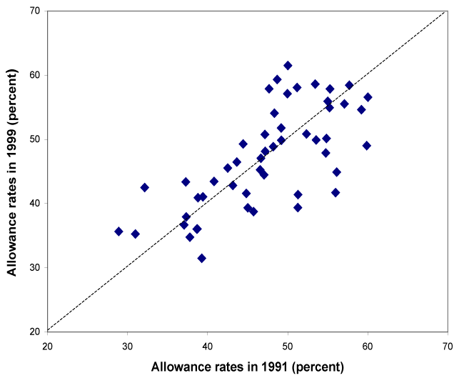
The variation in DI and SSI allowance rates across states has been substantial and persistent. Recently, the range between the states with the highest allowance rates and the ones with the lowest was around 30 percentage points.1 In addition, the states with the lowest allowance rates tend to remain in this category in adjacent years. Over longer periods of time, the ranking of allowance rates remains fairly stable. For example, Chart 1 plots DI allowance rates that are 8 years apart. States tend to keep their position relative to the other states, as shown by the proximity of the data points to the diagonal line.2
The stability of state DI allowance rates across years, 1991–1999
Even though the differences between allowance rates are large and persistent, an internal Social Security Administration study (1988) showed that much of the variation is associated with economic and demographic differences in state populations. The analysis also concluded that more variation could have been accounted for had data on additional factors (such as health) been available. Numerous other studies have analyzed the relationship between allowance rates and economic and demographic factors.3
This study expands on the 1988 analysis by considering a wider range of possible explanatory variables. It differs from previous studies by analyzing 3 years of data and by conducting separate analyses for the DI and SSI programs and for concurrent claims under both programs. It responds to concerns about differing allowance rates by reexamining the portion that is associated with external factors and, by extension, the portion that could be attributable to inconsistency. The analysis addresses the issue of whether a claimant in one state is less likely to be allowed than a claimant in another state, all other things being equal. By adjusting the allowance rates to account for demographic and economic conditions, this analysis moves toward making at least some important "other things" equal.
This study pertains to the average initial allowance rate for each state across all cases. Therefore, it does not reach any conclusions about the extent of variation across particular categories of disability or particular steps in the process. It also does not cover the important issue of possible inconsistency among decisionmakers within a state.
Factors Influencing Allowance Rates
This study aims to account for state-to-state differences in allowance rates using variables that are clearly external to the administration of the disability program. Variables that measure aspects of the economy or the population are in this category. An example is the age of the population; it is logical to expect higher allowance rates with an older population. The only variable used in the analysis that could be considered partially internal to the program is the percentage of applications based on physical (as opposed to mental) impairments. It is internal in the sense that it refers to a characteristic of the claimant rather than of the population. Although this variable is largely independent of the claims process, an element of subjective judgment exists in the classifying of disability cases. The analysis nevertheless uses this variable because there is no corresponding characteristic that can be measured in the state population.
One of the goals of this analysis is to separate the variation that can be influenced by administrative factors or policy from that which is attributable to external differences between states. Through controlling for the external factors for which data are available, the analysis can focus on the remaining differences in allowance rates.4
This study uses data for calendar years 1997, 1998, and 1999 to explain differences in allowance rates. It combines 3 years of data into a single analysis. In addition to allowing for greater statistical precision, combining the data permits an examination of whether anomalies recur in different years. Separate analysis is conducted for three different groups: DI claims, SSI claims, and concurrent claims under both programs.5 DI and SSI allowance rates can differ greatly in a particular state. The states with the lowest DI allowance rates do not necessarily have the lowest SSI allowance rates. Furthermore, DI and SSI filing rates are correlated with different external variables. Concurrent applicants represent a unique population with labor force experience but little financial success. This group has enough work experience to be insured for DI but has meager enough assets and income to qualify for SSI. Because of these differences, we separated the programs for the purpose of this analysis.
Candidate Explanatory Variables
This section discusses the variables that were considered for inclusion in the analysis based on prior expectations about what variables might be important. Some variables that would be expected to be important are, nevertheless, not included in the analysis for reasons discussed below.
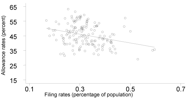
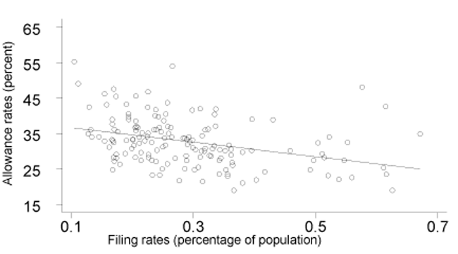
Filing Rates. Filing rates are the number of initial applications expressed as a percentage of the working-age population. Filing rates are negatively correlated with allowance rates; that is, the states with higher filing rates tend to have lower allowance rates, although not in all cases. Charts 2 and 3 plot data points for filing rates and allowance rates. The lines show the general relationship between the two.
DI filing rates and allowance rates, 1997–1999
SSI filing rates and allowance rates, 1997–1999
It is not essential to include filing rates in equations explaining allowance rates because filing rates themselves are heavily influenced by economic and demographic factors. The influences on filing rates are shown by regression equations in Appendix B. Although these equations employ additional variables, they also use the same or similar economic and demographic variables as are used to predict allowance rates. Thus, the influence of filing rates on allowance rates is also captured by these other variables. Consequently, when predicting allowance rates, filing rates have only a marginal effect. Filing rates are, nevertheless, included in the equations explaining allowance rates because readers may be curious about their impact.
Economic Indicators. Although filing rates are influenced by economic factors, the economic indicators have an independent effect on allowance rates even when controlling for filing rates. According to economic theory, deteriorating economic conditions influence some people to switch from the labor market to disability insurance for their primary means of support as their probability of success in the labor market declines. Thus, poorer economic conditions are associated both with higher filing rates on an aggregate level and with an applicant pool containing people with less severe impairments. If the medical judgments are consistent, one would expect that more people in this group would be denied benefits, resulting in lower allowance rates. Thus, economic conditions affect both allowance rates and filing rates.
Different aspects of economic conditions can be captured by different variables. The available candidate variables are the unemployment rate, the labor force participation rate, the poverty rate, per capita income, and the proportion employed in retail or wholesale trade.6
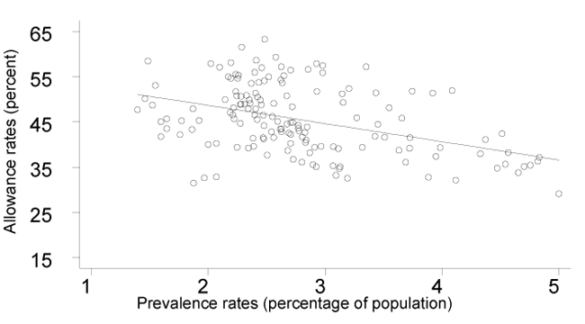
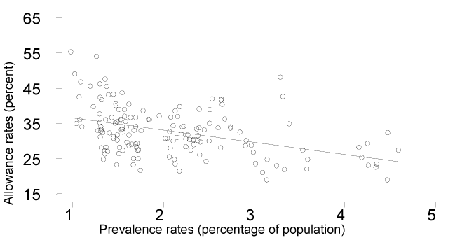
Prevalence Rates. The proportions of DI and SSI beneficiaries in the population, known as prevalence rates, are related to the allowance rates for DI and SSI, as shown in Charts 4 and 5. Despite the apparent relationship, prevalence rates are not good explanatory variables for allowance rates when the other economic and demographic variables have been included. This is because both prevalence rates and allowance rates are influenced by economic and demographic factors. Also, the prevalence rate and the allowance rate are conceptually related measures. In an accounting sense, a prevalence rate is the sum of many years' allowances and rates of leaving the programs.
DI prevalence rates and allowance rates, 1997–1999
SSI prevalence rates and allowance rates, 1997–1999
Demographic Indicators. Different demographic groups have different risks of disability. Demographic indicators include the median age, the proportion of the workforce in ages most vulnerable to disability, the percentage of the workforce that is male, and the percentage of the workforce that has a high school education.
Health Indicators. Previous reports, including one by the Social Security Administration (1988), referred to average health status by state as a crucial but, at the time, unavailable piece of data. Such data are now available through surveys measuring self-reported health and disability levels. Indeed, these indicators are important variables in predicting filing rates but are not essential for predicting allowance rates. Other health-related variables that are useful for explaining allowance rates include the proportion of workers with health insurance and the rate of nonfatal work-related injuries and illness.
Predictive Equations
The sets of variables described above are used in a regression analysis to examine the variation in allowance rates. Regression analysis is a statistical tool that divides the variation in a variable into explained and unexplained portions based on a set of predictor variables. A subset of the candidate variables described above was used in each equation. A combination of variables was selected based on the proportion of variation that was explained and the relevance of the variables to economic theory. The equations that were selected are not uniquely superior by any one criterion but are among a number of equations showing similar results. More information about the equations is given in Appendix B and Table B-3.
The equation for allowance rates among DI applicants contains the following variables:
- the filing rate,
- the percentage of applicants claiming physical disabilities,
- the percentage of the workforce with a high school education,
- the percentage of the workforce that is male,
- the occupational illness and injury rate,
- the median age of the population,
- per capita disposable income,
- the poverty rate,
- variables capturing the percentage of employment in industries with high injury and illness rates, and
- a variable capturing differences between years in the data.
The equation for allowance rates among SSI applicants contains the following variables:
- the filing rate,
- the percentage of applicants claiming physical disabilities,
- the percentage of the workforce with a high school education,
- the percentage of the workforce that is male,
- the median age of the population,
- the unemployment rate,
- the percentage of employment in retail trade,
- per capita disposable income,
- the percentage of workers with health insurance,
- variables capturing the percentage of employment in industries with high injury and illness rates, and
- two variables capturing differences between years in the data.
The equations for SSI and DI are similar. Both equations include the filing rate, the percentage of applicants claiming physical disabilities, the demographic variables, and the variables representing the composition of employment by industry. The equation for concurrent applicants is similar to the ones for DI and SSI and resembles a combination of the two. It contains the following variables:
- the filing rate,
- the percentage of applicants claiming physical disabilities,
- the percentage of the workforce with a high school education,
- the percentage of the workforce that is male,
- the median age of the population,
- the percentage of workers with health insurance,
- the unemployment rate,
- the poverty rate,
- the percentage of employment in retail trade,
- variables capturing the percentage of employment in industries with high injury and illness rates, and
- a variable capturing differences between years in the data.
In assessing studies such as this one, there is frequently concern that some of the explanatory variables are internal to the claims evaluation process. For example, although filing rates may be expected to influence allowance rates, the inverse may also be true. Allowance rates may influence filing rates if the population in particularly lenient or stringent states changes their filing behavior. Thus, it is uncertain whether a variable measuring the filing rate captures differences in a state's population or differences in the application of the disability standards. Appendix B illustrates the impact of the variables to which this critique would most apply, presenting empirical analysis both including and excluding these variables. The primary result is that including variables such as the filing rate makes little difference in the explanatory power of the model equations and the overall conclusions of the report. However, the results for an individual state and the identification of an individual state as a statistical outlier are affected by changing the variables of analysis.
The argument that certain variables measuring an aspect of the population may also capture variation in the claims evaluation process can potentially be extended to any of the explanatory variables. It is sometimes argued, for example, that adjudicators are more lenient during recessions. Following this logic, such variables as the unemployment rate or the poverty rate may capture an element of adjudicator judgment and may thus be internal to the claims evaluation process.7 It is beyond the scope of this paper to address the issue of whether adjudicators are more lenient during recessions. Variables such as the unemployment rate and the poverty rate remain in the analysis. Retaining these variables would create a problem in the analysis only if adjudicator leniency varies with economic conditions in a way that creates differences across states. There is no problem if leniency varies only with national economic trends rather than with state-level economic conditions.
In summary, regression equations are used to divide the variation in allowance rates into the portion associated with external variables and a remaining portion. This remaining portion is the difference between the predicted allowance rates calculated from the equations and actual allowance rates. The remaining portion is examined in the next section. This remaining portion is of particular interest, since it represents the portion of variation that could contain the effects of inconsistency in evaluating claims.
Actual and Predicted Allowance Rates
A predicted allowance rate was calculated for each year of analysis for SSI, DI, and concurrent applicants and is presented in Appendix C. This allowance rate reflects the rate that is expected given the demographic characteristics, economic indicators, and other variables used in each equation. The difference between the predicted allowance rate and the actual allowance rate represents the unexplained portion of the variation in allowance rates. States with the highest DI allowance rates in 1998 and their deviations are shown in the following tabulation:
| State | Actual allowance rate |
Predicted allowance rate |
Actual less predicted |
Actual less national mean |
|---|---|---|---|---|
| New Hampshire | 56.4 | 57.0 | -0.6 | 22.5 |
| Nevada | 56.9 | 47.1 | 9.8 | 23.0 |
| Minnesota | 57.1 | 58.8 | -1.8 | 23.2 |
| Vermont | 57.4 | 54.0 | 3.4 | 23.5 |
| Iowa | 63.3 | 51.5 | 11.8 | 29.4 |
Although these states all have high actual allowance rates, only some of them differ substantially from the predicted rate. These differences from predicted allowance rates were examined from the perspective of their likely occurrence due solely to random variability and analyzed in terms of the standard deviation of the predictive model.8 In Nevada, for example, there is a difference of 9.8 percentage points between the actual and predicted allowance rates for 1998. This difference exceeds two standard deviations (8.26 percentage points), so the Nevada allowance rate can be considered an outlier in 1998. The allowance rate for Iowa is also an outlier in 1998 whereas the other states listed here are not.9
Outlier Patterns
Three equations with 3 years of data for 50 states plus the District of Columbia provide 459 comparisons of actual and predicted allowance rates. Of these, 20 have differences from the predicted value in excess of two standard deviations, which is about 4.4 percent of observations; that is to be expected and is no cause for concern, in itself.
We now look for patterns of outliers in individual states. About half the outliers are a single occurrence for that state. In other words, the state is an outlier in 1 year of analysis but not in the other 2. A few states have more than one outlier. Out of a possible total of nine (three equations times 3 years), no state has more than four. The following tabulation shows states with more than one outlier:
| State | Number of outliers | Direction of outliers |
|---|---|---|
| Nevada | 4 | + |
| Hawaii | 3 | +/– |
| Wyoming | 2 | – |
| Arizona | 2 | + |
| NOTE: ( – ) indicates that the actual rate is lower than predicted; ( + ) indicates that the actual rate is higher than predicted. | ||
Other Patterns of Differences
No individual state is an outlier for all 3 years of analysis for any one set of applicants (SSI, DI, or concurrent applicants). In some states, however, there appears to be a pattern in the differences between actual and predicted allowance rates, even though the differences are less than two standard deviations. These patterns emerge when examining states that differ from their predicted value by at least one standard deviation.
The states that have differences that are greater than one standard deviation in all 3 years of analysis for one or more sets of applicants are listed in the tabulation below. A positive sign means the actual rate is higher than the predicted rate and vice versa. For example, the actual SSI allowance rate for Colorado is consistently lower than the predicted rate. The difference is 5.5, 6.5, and 11.0 percentage points for 1997, 1998, and 1999, respectively. Only the last figure is greater than two standard deviations, yet the available data consistently overpredict the SSI allowance rate for Colorado.
States that differ from the predicted value by more than one standard deviation for one set of applicants for all 3 years of analysis are as follows:
| SSI | DI | Concurrent applicants |
|---|---|---|
| Colorado – | Iowa + | Colorado – |
| Hawaii +/– | North Carolina + | Delaware + |
| Wyoming – | Maryland – | |
| NOTE: ( – ) indicates that the actual rate is lower than predicted; ( + ) indicates that the actual rate is higher than predicted. | ||
Discussion
If all states were the same in terms of their population and economy, it might be appropriate to expect them to have allowance rates near the national allowance rate. In that case, a measure of the extent of inconsistency in the application of the national disability criteria would be the difference between state allowance rates and the national mean.
Given economic and demographic differences among states, however, it is not appropriate to expect allowance rates to be the same. The difference between a state's actual and predicted allowance rates is a more appropriate measure of the extent to which the state might be applying national disability criteria differently than other states. Of course, this measure is dependent upon the quality of the available data as well as the choices made when constructing the regression equations. The measures are likely to capture the maximum difference that could be attributable to inconsistency since there are other aspects of the differences in caseloads that are not captured by the variables that were used.
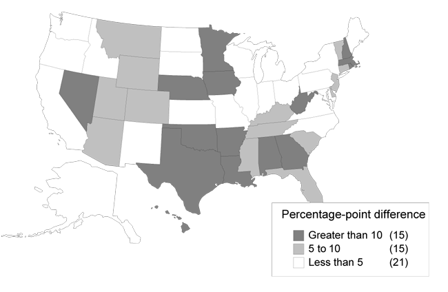
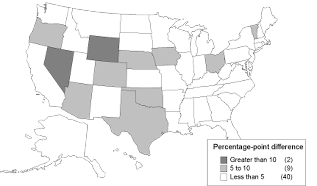
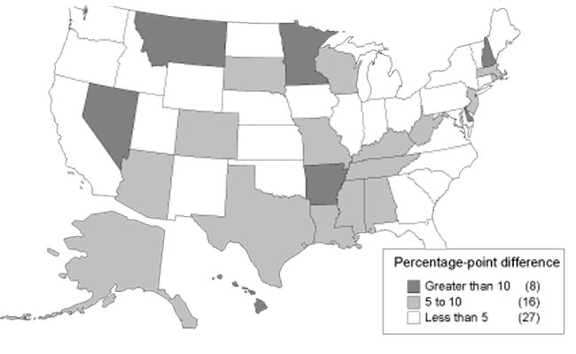
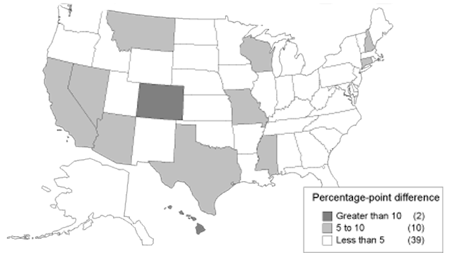
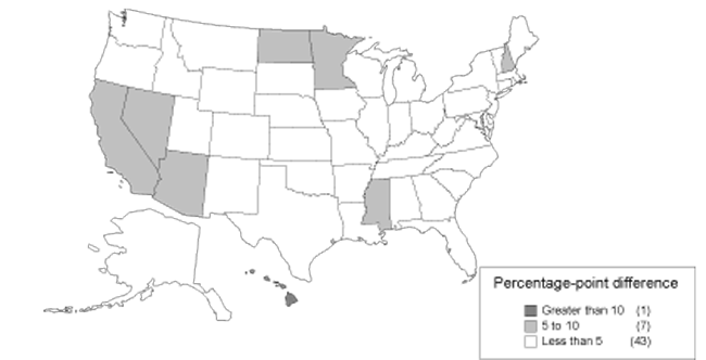
Comparisons between actual and predicted allowance rates are given for each state and year in Appendix C. The differences are presented visually in Charts 6, 7, 8, and 9. The states are divided into categories, with darker shades representing categories with greater differences. Chart 6 shows the differences between allowance rates and the mean for DI. It shows a concentration of large differences in the South. By contrast, Chart 7 shows the differences between allowance rates and predicted allowance rates. When accounting for economic and demographic differences by using predicted allowance rates, the South no longer exhibits a concentration of large differences. Similarly, Charts 8 and 9 show the same information for SSI. For both SSI and DI, there are fewer states with the darkest shade representing differences greater than 10 percentage points when comparing allowance rates with predicted allowance rates. For example, 15 states fall into this category in Chart 6, while only 2 remain in Chart 7. The remaining states correspond in large part to the states that were described as statistical outliers in the previous section. Nevada, Wyoming, and Hawaii also appear in the category representing the largest differences for either DI or SSI.
Absolute difference between DI allowance rates and the mean, 1999
Absolute difference between DI allowance rates and predicted values, 1999
Absolute difference between SSI allowance rates and the mean, 1999
Absolute difference between SSI allowance rates and predicted values, 1999
Because only a few states have large differences, a more representative picture of the magnitude of state variation emerges by examining differences for a typical state. The best way to show such differences is with the mean of the absolute differences. A typical state's DI allowance rate differs from the mean in either direction by 6.7 percentage points on average. It differs from the predicted rate by less than half that amount, however, only 3.1 percentage points. The reductions in allowance rate differences are not as notable for SSI or for concurrent applicants. These differences, in percentage points, are shown in the tabulation below, and more information is given in Appendix B.
| DI | SSI | Concurrent applicants | |
|---|---|---|---|
| Difference from mean | 6.7 | 5.6 | 4.5 |
| Difference from predicted value | 3.1 | 3.2 | 3.0 |
Conclusion
A major concern regarding the quality of disability adjudication has been the consistency of decisions. While no two cases are identical, SSA seeks to ensure that criteria are applied consistently and that like cases will have the same outcome. This study has focused on a subset of that issue—the variation in allowance rates across states. The difference between a typical state's allowance rate and its predicted allowance rate (for example, adjusted for economic, demographic, and health factors) is estimated to be about half the difference between a typical state's allowance rate and the national mean. Nonetheless, differences still exist, and a few states have DI or SSI allowance rates that are consistently above or below their predicted rates. By focusing on areas of real rather than apparent inconsistency, SSA can more effectively focus future examination of the issue of inconsistency.
Appendix A
| State | Actual allowance rate | Predicted allowance rate |
|---|---|---|
| DI allowance rates | ||
| Lowest | ||
| West Virginia | 29.1 | 29.4 |
| Alabama | 32.2 | 35.7 |
| Louisiana | 32.5 | 27.3 |
| Texas | 32.9 | 33.2 |
| Oklahoma | 33.2 | 33.5 |
| Highest | ||
| Maine | 51.9 | 46.5 |
| Vermont | 52.3 | 45.4 |
| Minnesota | 55.0 | 57.6 |
| South Dakota | 55.2 | 49.7 |
| Iowa | 57.2 | 50.8 |
| SSI allowance rates | ||
| Lowest | ||
| Arkansas | 18.9 | 24.0 |
| West Virginia | 18.9 | 18.3 |
| Missouri | 21.4 | 24.8 |
| Montana | 21.6 | 22.4 |
| Alabama | 21.9 | 19.7 |
| Highest | ||
| Washington | 36.2 | 33.5 |
| Massachusetts | 36.2 | 33.6 |
| Delaware | 40.5 | 35.5 |
| New Hampshire | 42.5 | 40.5 |
| Minnesota | 43.1 | 39.2 |
| Concurrent allowance rates | ||
| Lowest | ||
| West Virginia | 16.6 | 19.5 |
| Alabama | 20.3 | 17.6 |
| Oklahoma | 20.4 | 21.7 |
| Arkansas | 20.5 | 24.7 |
| New Mexico | 20.7 | 24.9 |
| Highest | ||
| Washington | 32.3 | 30.9 |
| Nevada | 33.4 | 32.4 |
| New Hampshire | 34.7 | 36.8 |
| Delaware | 38.4 | 32.9 |
| Minnesota | 38.7 | 35.9 |
| State | Actual allowance rate | Predicted allowance rate |
|---|---|---|
| DI allowance rates | ||
| Lowest | ||
| Texas | 32.6 | 37.7 |
| Alabama | 32.7 | 39.6 |
| Arkansas | 33.7 | 33.3 |
| Oklahoma | 35.1 | 41.0 |
| Louisiana | 35.1 | 34.1 |
| Highest | ||
| New Hampshire | 56.4 | 57.0 |
| Nevada | 56.9 | 47.1 |
| Minnesota | 57.1 | 58.8 |
| Vermont | 57.4 | 54.0 |
| Iowa | 63.3 | 51.5 |
| SSI allowance rates | ||
| Lowest | ||
| Arkansas | 21.0 | 23.4 |
| Alabama | 23.0 | 26.4 |
| Mississippi | 23.1 | 23.1 |
| West Virginia | 23.4 | 25.1 |
| Missouri | 24.7 | 28.1 |
| Highest | ||
| District of Columbia | 42.6 | 45.5 |
| Delaware | 43.2 | 40.4 |
| Nevada | 45.5 | 37.0 |
| Minnesota | 47.5 | 41.7 |
| New Hampshire | 49.0 | 47.7 |
| Concurrent allowance rates | ||
| Lowest | ||
| Arkansas | 21.1 | 21.0 |
| Alabama | 21.4 | 24.4 |
| Montana | 21.6 | 25.5 |
| West Virginia | 22.7 | 25.1 |
| Missouri | 23.7 | 25.0 |
| Highest | ||
| Arizona | 36.7 | 33.9 |
| Delaware | 39.3 | 34.5 |
| Minnesota | 39.9 | 37.5 |
| Nevada | 40.5 | 34.1 |
| New Hampshire | 42.5 | 41.0 |
| State | Actual allowance rate | Predicted allowance rate |
|---|---|---|
| DI allowance rates | ||
| Lowest | ||
| Texas | 31.5 | 38.4 |
| Arkansas | 34.8 | 34.5 |
| Louisiana | 35.3 | 35.8 |
| West Virginia | 35.7 | 35.5 |
| Alabama | 36.0 | 38.6 |
| Highest | ||
| Nebraska | 58.1 | 50.7 |
| Hawaii | 58.5 | 54.4 |
| Iowa | 58.6 | 52.9 |
| New Hampshire | 59.3 | 56.4 |
| Nevada | 61.5 | 48.5 |
| SSI allowance rates | ||
| Lowest | ||
| Montana | 23.2 | 30.7 |
| Arkansas | 23.5 | 25.8 |
| Alabama | 24.7 | 25.3 |
| West Virginia | 25.3 | 24.7 |
| Missouri | 25.4 | 30.9 |
| Highest | ||
| Minnesota | 46.1 | 41.7 |
| Nevada | 46.7 | 39.5 |
| District of Columbia | 48.1 | 46.9 |
| Hawaii | 54.0 | 43.3 |
| New Hampshire | 55.3 | 50.1 |
| Concurrent allowance rates | ||
| Lowest | ||
| Montana | 20.9 | 27.3 |
| Arkansas | 21.9 | 24.7 |
| West Virginia | 21.9 | 25.9 |
| Alabama | 23.6 | 23.6 |
| Texas | 24.0 | 28.4 |
| Highest | ||
| Minnesota | 41.1 | 37.0 |
| District of Columbia | 41.3 | 35.3 |
| New Hampshire | 43.1 | 39.8 |
| Hawaii | 44.2 | 36.5 |
| Nevada | 45.7 | 36.5 |
Appendix B: Technical Notes
This appendix presents the results of the regression analysis and discusses topics relevant to their interpretation. Interpretation of the influences on allowance rates is aided by discussion of the influences on filing rates; thus a discussion of filing behavior and an empirical analysis of filing rates is presented first. The analysis of allowance rates follows.
Filing Rates
Interpretation of the equations in this paper is aided by two assumptions about individual choice and the nature of disability. First, according to standard economic theory, people choose rationally between alternatives. In this case, the relevant alternatives are seeking work and filing for disability. It follows that the decision of those at the margin is affected by the return to each choice, in this case the size of the disability payment and the attainable wage from employment. Economic indicators serve as a proxy for the attainable wage, in aggregate.10 Second, the analysis assumes that disability status itself is not affected by economic conditions, at least in the short run. Poverty and unemployment may affect the onset of disability through nutrition, safety, and other influences; however, this presumably happens gradually. Taken together, these two points portray filing behavior as more responsive to economic conditions and disability itself as less responsive. Therefore, when analyzing allowance rates, the effect of changing economic conditions is largely through changes in filing behavior and, it follows, in the composition of the applicant pool. The composition of the applicant pool is hypothesized to be one of the determining factors for aggregate allowance rates.
It follows that the interpretation of allowance rates rests in part on the interpretation of filing behavior. There is substantial empirical evidence that filing behavior changes in response to changing conditions. Leonard (1986) reviews the studies that examine whether changes in the DI benefit amounts affect the tendency to work. The consensus is that they do, although the magnitudes of the estimated effects vary widely. Conversely, various chapters in Rupp and Stapleton (1998) review and contribute to the literature on whether changes in the reward to work affect filing behavior. Again, the results point to substantial effects.
The results of this paper agree with most previous studies. Table B-1 shows some simple evidence about the influences on filing rates. The regressions describe filing rates for DI and SSI and include concurrent applicants. All the independent variables described in the text were made available for these regressions. Around 80 percent of the variation can be described with just a few variables, although different variables appear in the DI and SSI equations. Not surprisingly, the poverty rate appears only in the SSI equation since only that program has a means test. The DI equation uses the labor force participation rate. The negative sign is consistent with a discouraged worker effect; as labor force participation declines, DI filings increase. Demographic variables that capture some behavioral differences across age and educational attainment categories are also used, as are the self-reported health and disability averages from the Current Population Survey. Self-reported disability is strongly correlated with filing for DI. The industry variables that are included are also intended to measure an aspect of health. They capture the percentage of employment in various industries that have relatively high occupational injury and illness rates.
| DI | SSI | |
|---|---|---|
| Percentage of workforce that is male | -0.01190* (0.00439) |
-0.02222* (0.00390) |
| Percentage of workforce completed high school | -0.00646* (0.00230) |
|
| Median age of population | 0.01571 (0.00807) |
|
| Labor force participation rate | -0.00598 (0.00314) |
|
| Poverty rate | 0.03065* (0.00274) |
|
| Disposable per capita income | -0.00555* (0.00276) |
|
| Percentage of employment in construction | 1.41154* (0.60388) |
|
| Percentage of employment in agriculture | 0.99811* (0.27196) |
|
| Percentage of employment in three industries a | 0.00532* (0.00185) |
|
| Percentage who say their health is poor | 0.03317* (0.00995) |
0.06733* (0.00641) |
| Percentage who say a disability prevents work | 0.02396* (0.00677) |
|
| Intercept | 1.22678* (0.49366) |
1.18277* (0.20629) |
| R-square | 0.7811 | 0.8488 |
| Root MSE | 0.07562 | 0.08083 |
| NOTE: * = statistically significant at the 5 percent level. Blank cell = variable not included. | ||
| a. Agriculture, construction, and manufacturing. | ||
Allowance Rates
Given these effects on filing rates, the pool of DI and SSI applicants changes with the economy and with demographic and health trends. The regression coefficients in the allowance rate equations are interpreted in this light. A procyclical economic indicator, for example, would be expected to have a positive sign. If per capita income falls during a recession, one would expect more marginal applicants to file for benefits. With the applicant pool diluted by these marginal filers, one would expect the allowance rate to be lower. Similarly, employment in retail trade is sometimes a good procyclical indicator of the low-wage labor market, but that is not borne out in these data. Countercyclical indicators such as the unemployment rate and the poverty rate are expected to have a negative sign.
The demographic variables have more straightforward interpretations. Disability is more prevalent at older ages and is associated with low educational achievement. The expected sign is thus positive for median age and negative for the percentage of the workforce that has completed high school. By contrast, there are no a priori expectations for the signs on the coefficients for percentage of the workforce that is male and percentage of applicants claiming a physical disability.
The remaining variables are related to health or occupational illness and injury. In general, one would expect health to be negatively associated with allowance rates. The variables representing employment in various industries capture employment in industries with high risk; agriculture, construction, manufacturing, and transportation are the one-digit Standard Industrial Classification codes with the highest rates of occupational illness and injury. These variables and the rate of occupational illness and injury itself are expected to have positive signs.
Tables B-2 and B-3 show two sets of regressions for the allowance rate equations. They differ primarily in terms of conceptual approach. The preliminary results shown in Table B-2 represent specifications reflecting a priori ideas about what variables should be included. By contrast, the final specifications in Table B-3 were chosen because they are among those that produce a good fit with just a few explanatory variables, within some limits. The fact that these two approaches produce quite similar results shows that the distinction between the two is not a crucial one. The regressions that are compatible with a priori ideas are close to the ones with a near-optimal fit. Similarly, the regressions with a near-optimal fit do not conflict with the a priori ideas. The results of the equations in Table B-3 were used for the analysis in the main text.
| DI | SSI | Concurrent | |
|---|---|---|---|
| Percentage of filings that are physical (not mental) | -0.89159* (0.16965) |
-0.69708* (0.09448) |
-0.57537* (0.08411) |
| Percentage of workforce completed high school | 0.28058* (0.12211) |
-0.25564 (0.13274) |
-0.24502* (0.10904) |
| Percentage of workforce that is male | -0.00952 (0.28680) |
0.53465* (0.26300) |
0.43943* (0.21561) |
| Median age of population | 1.31307* (0.50479) |
0.19214 (0.44618) |
0.58091 (0.37650) |
| Unemployment rate | -1.73610* (0.49489) |
-1.14526* (0.40036) |
|
| Poverty rate | -0.79708* (0.24673) |
0.53526* (0.21573) |
|
| Disposable per capita income | 0.59555* (0.21626) |
0.83126* (0.22507) |
0.34152 (0.18715) |
| Percentage of employment in retail trade | 98.00137 (388.051) |
1052.944* (353.679) |
685.3652* (294.989) |
| Percentage of employment in four industries a | -1.65705* (0.64320) |
-1.81342* (0.62828) |
-2.55525* (0.53724) |
| Percentage of employment in four industries squared | 0.02456 (0.01409) |
0.03271* (0.01389) |
0.04837* (0.01162) |
| Nonfatal occupational injury and illness rate | 1.70638* (0.48998) |
-0.27725 (0.45141) |
0.17414 (0.37774) |
| Percentage of workers with health insurance | -0.07398 (0.14250) |
-0.58860* (0.14502) |
-0.52298* (0.11904) |
| Year is 1997 | -1.15364 (1.05677) |
-2.22333* (0.97163) |
-2.21296* (0.82236) |
| Year is 1998 | -1.15364 (1.05677) |
1.24468 (0.89852) |
-0.23165 (0.73330) |
| Intercept | 59.50867 (37.3423) |
112.2613* (39.4099) |
114.1173* (33.6754) |
| R-square | 0.6395 | 0.6485 | 0.6196 |
| Root MSE | 4.71286 | 4.27906 | 3.52434 |
| NOTE: * = statistically significant at the 5 percent level. Blank cell = variable not included. | |||
| a. Agriculture, construction, manufacturing, and transportation. | |||
| DI | SSI | Concurrent | |
|---|---|---|---|
| Filing rate (percent) | 7.39238 (6.45851) |
-18.6228* (4.91978) |
-0.02463 (4.15680) |
| Percentage of filings that are physical (not mental) | -1.20631* (0.14799) |
-0.81912* (0.08777) |
-0.72378* (0.09362) |
| Percentage of workforce completed high school | -0.29838* (0.14482) |
-0.48208* (0.12571) |
-0.34014* (0.11592) |
| Percentage of workforce that is male | 0.47068* (0.23106) |
0.61456* (0.23956) |
0.40772 (0.22441) |
| Median age of population | 1.29464* (0.47063) |
0.55066* (0.41318) |
0.81724* (0.35558) |
| Unemployment rate | -1.31473* (0.48700) |
-1.87899* (0.42773) |
|
| Poverty rate | -0.86872* (0.19953) |
-0.52263* (0.20810) |
|
| Disposable per capita income | 0.44462* (0.20318) |
0.91493* (0.15657) |
|
| Percentage of employment in retail trade | 624.32458 (330.261) |
180.07423 (264.372) |
|
| Percentage of employment in agriculture | 122.2299* (19.2863) |
-86.0791* (25.5015) |
|
| Percentage of employment in manufacturing | -82.0571* (22.2779) |
||
| Percentage of employment in three industries a | -2.45914* (0.45926) |
||
| Percentage of employment in three industries squared | 0.05121* (0.01190) |
||
| Percentage of employment in four industries b | -1.90453* (0.58265) |
-3.12508* (0.43983) |
|
| Percentage of employment in four industries squared | 0.02589* (0.01291) |
0.07648* (0.01091) |
|
| Nonfatal occupational injury and illness rate | 1.19549* (0.42092) |
||
| Percentage of workers with health insurance | -0.55047* (0.13026) |
-0.47814* (0.11729) |
|
| Year is 1997 | -2.61184* (0.77473) |
-1.62384 (0.90238) |
2.08065* (0.65209) |
| Year is 1998 | -1.61386* (0.81459) |
||
| Intercept | 120.7340* (28.6846) |
126.0639* (32.7617) |
150.8526* (29.9893) |
| R-square | 0.7213 | 0.7069 | 0.6457 |
| Root MSE | 4.12922 | 3.90767 | 3.40142 |
| NOTE: * = statistically significant at the 5 percent level. Blank cell = variable not included. | |||
| a. Agriculture, construction, and manufacturing. | |||
| b. Agriculture, construction, manufacturing, and transportation. | |||
There were several a priori considerations in the variable selection for Table B-2. Variables were selected corresponding to the nature of the SSI and DI programs. The poverty rate was employed as a predictor for the SSI equation corresponding to the SSI means test, whereas the unemployment rate has a rough relation to the work history requirement for DI eligibility.
Another consideration for Table B-2 was to exclude variables that contained possible endogeneity. As demonstrated above, most of the variation in filing rates corresponds to economic and demographic differences among states. However, it is possible that filing rates also respond to state differences in program administration. For example, states with more allowances could inspire additional people to file for benefits. It is also possible that some predictor variables are coincidentally correlated with adjudicative, administrative, or policy differences. Industry employment indicators, for example, could capture variations that correspond to such differences.11 Because of this, the filing rate was excluded, and industry variables were included only in aggregated form in Table B-2.
The variables in Table B-3, by contrast, were selected with less regard for these issues. These equations were selected on the basis that they explain a large amount of the variation with relatively few variables. Variables were generally excluded if they did not contribute to the overall fit. The selection does not represent a complete disregard for endogeneity issues, however. The variables that are most likely to be endogenous have been excluded. For example, the average levels of self-reported health and disability were categorically excluded from these equations. The evidence indicates that the remaining variables are primarily exogenous but could be contaminated by some endogeneity.
The relevance of this issue is limited by the size of the differences between the two sets of equations. Given that the results are similar, including a few potentially marginally endogenous variables cannot undermine the results significantly. The results are similar in several ways. The signs and magnitudes of the coefficients that are included in both sets of equations are similar, with only one exception for both the sign (percentage completing high school) and the magnitude (percentage of employment in retail trade) in three equations. Also, the explained portion of the variation is similar, and the two sets of equations produce similar sets of outliers. The rank order correlations of the regression residuals are 0.83, 0.91, and 0.94 for DI, SSI, and concurrent applicants, respectively.
The outliers from the regressions in Table B-2 are shown in Charts 11 and 13. (To facilitate comparison, Charts 6 and 8 are repeated here as Charts 10 and 12.) In some cases, the two sets of equations produce different outliers. Thus, the results for any one particular state depend on the choice of specification; however, the overall results are independent of the choice of specification.
Absolute difference between DI allowance rates and the mean, 1999
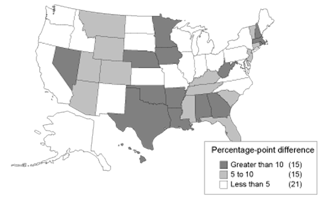
Absolute difference between DI allowance rates and predicted values, 1999
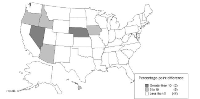
Absolute difference between SSI allowance rates and the mean, 1999
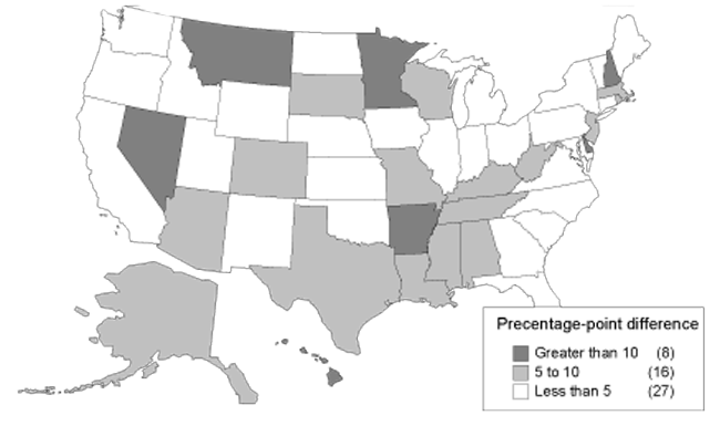
Absolute difference between SSI allowance rates and predicted values, 1999
The signs in Tables B-2 and B-3 are generally as expected. The coefficient on the percentage of filings that are physical is negative, indicating that physical claims have a lower allowance rate than mental claims. States with more males in the workforce and a higher median age have higher allowance rates. The coefficients for cyclical and health indicators have the signs discussed above. The coefficients for filing rates are negative but generally not statistically significant. It is not essential to include filing rates in the equation when the economic and health variables that are highly correlated with filing rates are included. Filing rates are included in Table B-3 because many readers may expect to see this effect.
Some other potential weaknesses of these equations should also be mentioned. The inclusion of filing rates illustrates that multicollinearity is present in these equations. Multicollinearity is a general problem not isolated to this variable. All the variables are related to deprivation of either health or income, and health and income are also correlated. Thus, the accuracy of the standard errors and tests of significance is affected. The worst cases of multicollinearity have been removed. For example, self-reported disability has a correlation with the DI filing rate of around 0.8 and is thus excluded from the DI allowance rate equations.
The predictive value of the equations is not affected, however. The predictions are the product of the data and the regression coefficients summed for each observation. Table B-4 shows the quantile distributions of the difference between actual allowance rates and the predictions (based on Table B-3), as well as the distribution of the differences from the mean. It shows that the variation in allowance rates by states is lower when accounting for the variation due to economic and demographic factors. The figures give a sense of how much lower the variation is than when using the mean as a basis for comparison. The differences from the predicted rates have a smaller range and a more compressed distribution. At any point in the distribution (the 5th percentile, for example), the differences between allowance rates and predicted rates are smaller than the differences between allowance rates and the mean. This is a measure of the composite predictive power of the independent variables. Smaller average differences and a smaller variability of differences result from taking the independent variables into account. This result is robust with respect to choice of specification and the potential problems mentioned above.
| DI | SSI | |||
|---|---|---|---|---|
| Difference from mean |
Difference from predicted value |
Difference from mean |
Difference from predicted value |
|
| Maximum | 14.4 | 13.0 | 20.6 | 10.7 |
| 95th percentile | 11.5 | 7.4 | 13.5 | 8.1 |
| 90th percentile | 10.8 | 5.2 | 10.7 | 5.2 |
| 75th percentile | 7.6 | 3.1 | 3.8 | 2.7 |
| Median | 0 | -0.1 | -1.3 | 0.2 |
| 25th percentile | -6.0 | -1.9 | -5.4 | -2.4 |
| 10th percentile | -11.0 | -3.9 | -7.4 | -5.1 |
| 5th percentile | -11.8 | -6.6 | -10.0 | -7.6 |
| Minimum | -15.6 | -10.2 | -11.5 | -10.7 |
| Mean | 0 | 0.2 | 0 | 0 |
| Mean of absolute value | 6.7 | 3.1 | 5.6 | 3.2 |
| Standard deviation | 7.9 | 4.2 | 7.3 | 4.2 |
It is also possible that using aggregate state-level data rather than individual-level data will introduce a bias in the estimates presented in this paper (see Robinson 1950 and Heckman 2001). Individuals within a state make the decision to apply for disability benefits, and individual adjudicators make a decision to award disability benefits. There is considerable within-state heterogeneity in economic and demographic factors. Aggregate-level data ignore this heterogeneity; thus the estimates presented in this paper may over- or underestimate the degree to which the variation is attributable to differences in environmental factors as opposed to the application of the SSA disability standard. Individual-level data may be examined in future work on this topic.
Appendix C
| State and year | SSI allowance rate | DI allowance rate | Concurrent allowance rate | ||||||
|---|---|---|---|---|---|---|---|---|---|
| Actual (percent) |
Predicted (percent) |
Deviation from predicted (percentage points) |
Actual (percent) |
Predicted (percent) |
Deviation from predicted (percentage points) |
Actual (percent) |
Predicted (percent) |
Deviation from predicted (percentage points) |
|
| Alabama | |||||||||
| 1997 | 21.9 | 19.7 | 2.2 | 32.2 | 35.7 | -3.5 | 20.3 | 17.6 | 2.6 |
| 1998 | 23.0 | 26.4 | -3.5 | 32.7 | 39.6 | -6.8 | 21.4 | 24.4 | -3.0 |
| 1999 | 24.7 | 25.3 | -0.5 | 36.0 | 38.6 | -2.6 | 23.6 | 23.6 | -0.1 |
| Alaska | |||||||||
| 1997 | 36.0 | 30.5 | 5.5 | 45.7 | 45.4 | 0.3 | 30.5 | 27.2 | 3.2 |
| 1998 | 41.7 | 39.8 | 1.9 | 48.7 | 51.0 | -2.3 | 34.2 | 34.6 | -0.4 |
| 1999 | 39.7 | 38.7 | 1.0 | 50.1 | 49.2 | 0.9 | 33.7 | 34.1 | -0.4 |
| Arizona | |||||||||
| 1997 | 34.0 | 33.7 | 0.3 | 43.9 | 39.9 | 3.9 | 30.3 | 30.8 | -0.5 |
| 1998 | 40.4 | 37.7 | 2.7 | 50.8 | 45.4 | 5.4 | 36.7 | 33.9 | 2.9 |
| 1999 | 43.7 | 35.6 | 8.1 | 54.9 | 46.6 | 8.3 | 39.1 | 34.1 | 4.9 |
| Arkansas | |||||||||
| 1997 | 18.9 | 24.0 | -5.1 | 35.4 | 29.4 | 6.0 | 20.5 | 24.7 | -4.3 |
| 1998 | 21.0 | 23.4 | -2.4 | 33.7 | 33.3 | 0.4 | 21.1 | 21.0 | 0.1 |
| 1999 | 23.5 | 25.8 | -2.3 | 34.8 | 34.5 | 0.3 | 21.9 | 24.7 | -2.8 |
| California | |||||||||
| 1997 | 28.1 | 30.2 | -2.1 | 40.3 | 42.4 | -2.1 | 26.5 | 23.4 | 3.0 |
| 1998 | 38.8 | 30.9 | 7.9 | 45.3 | 46.0 | -0.7 | 30.2 | 27.0 | 3.2 |
| 1999 | 39.0 | 32.6 | 6.4 | 47.9 | 47.1 | 0.8 | 32.9 | 28.2 | 4.7 |
| Colorado | |||||||||
| 1997 | 26.3 | 31.9 | -5.5 | 39.6 | 42.8 | -3.2 | 24.4 | 28.9 | -4.5 |
| 1998 | 27.2 | 33.7 | -6.5 | 39.2 | 45.6 | -6.4 | 24.1 | 28.8 | -4.7 |
| 1999 | 28.1 | 38.7 | -11.0 | 39.4 | 45.5 | -6.2 | 25.5 | 31.2 | -5.8 |
| Connecticut | |||||||||
| 1997 | 26.4 | 30.1 | -3.8 | 48.7 | 50.6 | -1.8 | 24.6 | 27.0 | -2.4 |
| 1998 | 31.7 | 39.5 | -7.8 | 53.7 | 55.3 | -1.6 | 30.2 | 35.2 | -5.0 |
| 1999 | 35.0 | 40.1 | -5.1 | 55.9 | 56.2 | -0.3 | 35.2 | 36.1 | -0.9 |
| Delaware | |||||||||
| 1997 | 40.5 | 35.5 | 5.0 | 51.7 | 49.5 | 2.2 | 38.4 | 32.9 | 5.5 |
| 1998 | 43.2 | 40.4 | 2.8 | 53.7 | 47.3 | 6.4 | 39.3 | 34.5 | 4.7 |
| 1999 | 45.4 | 43.6 | 1.8 | 54.1 | 49.6 | 4.5 | 41.0 | 32.4 | 8.6 |
| District of Columbia | |||||||||
| 1997 | 34.8 | 39.5 | -4.6 | 48.9 | 50.6 | -1.7 | 30.3 | 33.7 | -3.4 |
| 1998 | 42.6 | 45.5 | -2.9 | 54.7 | 54.8 | -0.1 | 35.0 | 35.5 | -0.5 |
| 1999 | 48.1 | 46.9 | 1.3 | 55.5 | 55.5 | 0.0 | 41.3 | 35.3 | 5.9 |
| Florida | |||||||||
| 1997 | 30.7 | 28.6 | 2.1 | 39.4 | 38.4 | 0.9 | 28.0 | 26.1 | 1.9 |
| 1998 | 37.1 | 31.6 | 5.4 | 39.5 | 41.0 | -1.5 | 30.5 | 28.3 | 2.3 |
| 1999 | 36.0 | 32.6 | 3.4 | 40.9 | 41.6 | -0.6 | 31.2 | 31.1 | 0.2 |
| Georgia | |||||||||
| 1997 | 27.4 | 24.7 | 2.7 | 34.7 | 34.0 | 0.7 | 23.8 | 22.5 | 1.4 |
| 1998 | 28.3 | 28.1 | 0.3 | 35.5 | 37.3 | -1.8 | 24.6 | 24.2 | 0.3 |
| 1999 | 31.0 | 28.2 | 2.8 | 36.7 | 37.5 | -0.8 | 26.5 | 25.7 | 0.7 |
| Hawaii | |||||||||
| 1997 | 27.0 | 31.5 | -4.5 | 45.1 | 47.4 | -2.3 | 22.3 | 29.8 | -7.5 |
| 1998 | 42.4 | 36.1 | 6.3 | 53.0 | 50.0 | 3.0 | 32.6 | 29.8 | 2.8 |
| 1999 | 54.0 | 43.3 | 10.7 | 58.5 | 54.4 | 4.0 | 44.2 | 36.5 | 7.7 |
| Idaho | |||||||||
| 1997 | 31.6 | 30.0 | 1.6 | 41.3 | 43.9 | -2.6 | 26.1 | 29.1 | -3.0 |
| 1998 | 35.8 | 36.5 | -0.7 | 46.5 | 48.0 | -1.5 | 33.0 | 31.3 | 1.8 |
| 1999 | 36.6 | 35.4 | 1.3 | 50.8 | 46.1 | 4.7 | 33.7 | 32.0 | 1.7 |
| Illinois | |||||||||
| 1997 | 30.0 | 28.4 | 1.6 | 44.7 | 43.2 | 1.5 | 29.5 | 24.4 | 5.1 |
| 1998 | 34.4 | 34.1 | 0.3 | 46.6 | 47.3 | -0.7 | 30.6 | 28.3 | 2.3 |
| 1999 | 32.6 | 35.2 | -2.5 | 47.1 | 46.7 | 0.4 | 30.7 | 29.4 | 1.2 |
| Indiana | |||||||||
| 1997 | 29.6 | 31.1 | -1.5 | 41.7 | 42.8 | -1.2 | 27.3 | 27.9 | -0.6 |
| 1998 | 34.0 | 36.8 | -2.9 | 44.9 | 43.7 | 1.3 | 31.9 | 34.6 | -2.7 |
| 1999 | 33.4 | 35.8 | -2.4 | 43.5 | 45.3 | -1.9 | 29.4 | 32.5 | -3.0 |
| Iowa | |||||||||
| 1997 | 35.5 | 34.4 | 1.1 | 57.2 | 50.8 | 6.4 | 31.7 | 31.1 | 0.6 |
| 1998 | 39.0 | 37.8 | 1.2 | 63.3 | 51.5 | 11.8 | 34.7 | 32.1 | 2.7 |
| 1999 | 36.1 | 36.7 | -0.5 | 58.6 | 52.9 | 5.8 | 31.1 | 32.4 | -1.3 |
| Kansas | |||||||||
| 1997 | 23.2 | 28.8 | -5.6 | 44.2 | 48.4 | -4.2 | 20.7 | 25.0 | -4.3 |
| 1998 | 30.7 | 30.2 | 0.5 | 53.5 | 48.2 | 5.3 | 26.9 | 26.0 | 0.8 |
| 1999 | 32.2 | 34.5 | -2.2 | 48.9 | 49.7 | -0.8 | 26.5 | 30.7 | -4.2 |
| Kentucky | |||||||||
| 1997 | 27.4 | 28.5 | -1.1 | 36.3 | 38.5 | -2.2 | 24.2 | 25.6 | -1.4 |
| 1998 | 32.3 | 33.1 | -0.7 | 42.4 | 42.4 | 0.0 | 29.2 | 30.0 | -0.8 |
| 1999 | 29.3 | 31.0 | -1.8 | 37.9 | 41.3 | -3.3 | 25.4 | 31.6 | -6.2 |
| Louisiana | |||||||||
| 1997 | 22.0 | 22.3 | -0.3 | 32.5 | 27.3 | 5.2 | 22.6 | 20.0 | 2.6 |
| 1998 | 24.7 | 26.7 | -2.0 | 35.1 | 34.1 | 1.0 | 24.6 | 24.1 | 0.5 |
| 1999 | 27.4 | 29.7 | -2.3 | 35.3 | 35.8 | -0.6 | 26.1 | 27.2 | -1.0 |
| Maine | |||||||||
| 1997 | 33.7 | 33.2 | 0.5 | 51.9 | 46.5 | 5.4 | 32.0 | 32.1 | -0.1 |
| 1998 | 35.0 | 38.8 | -3.8 | 51.4 | 50.9 | 0.5 | 31.0 | 33.3 | -2.3 |
| 1999 | 33.7 | 36.7 | -3.1 | 51.8 | 51.1 | 0.7 | 30.4 | 33.3 | -2.9 |
| Maryland | |||||||||
| 1997 | 28.2 | 29.4 | -1.3 | 40.0 | 46.5 | -6.4 | 24.3 | 28.7 | -4.4 |
| 1998 | 30.3 | 35.0 | -4.7 | 43.3 | 49.0 | -5.7 | 26.5 | 33.4 | -6.9 |
| 1999 | 31.2 | 33.5 | -2.3 | 45.3 | 48.5 | -3.2 | 27.5 | 33.7 | -6.2 |
| Massachusetts | |||||||||
| 1997 | 36.2 | 33.6 | 2.6 | 51.2 | 48.2 | 3.0 | 31.2 | 32.8 | -1.6 |
| 1998 | 41.9 | 36.6 | 5.3 | 55.9 | 51.2 | 4.7 | 34.3 | 34.3 | 0.0 |
| 1999 | 40.4 | 39.2 | 1.2 | 57.9 | 54.7 | 3.2 | 34.7 | 37.2 | -2.6 |
| Michigan | |||||||||
| 1997 | 30.4 | 28.3 | 2.1 | 40.5 | 44.3 | -3.8 | 29.0 | 27.3 | 1.7 |
| 1998 | 31.7 | 30.8 | 0.9 | 40.2 | 46.3 | -6.1 | 28.4 | 30.3 | -1.8 |
| 1999 | 31.9 | 32.5 | -0.6 | 43.4 | 47.3 | -3.9 | 30.3 | 30.9 | -0.6 |
| Minnesota | |||||||||
| 1997 | 43.1 | 39.2 | 3.9 | 55.0 | 57.6 | -2.6 | 38.7 | 35.9 | 2.8 |
| 1998 | 47.5 | 41.7 | 5.8 | 57.1 | 58.8 | -1.8 | 39.9 | 37.5 | 2.3 |
| 1999 | 46.1 | 41.7 | 4.5 | 57.9 | 58.4 | -0.5 | 41.1 | 37.0 | 4.1 |
| Mississippi | |||||||||
| 1997 | 22.5 | 16.4 | 6.1 | 37.2 | 30.0 | 7.2 | 23.0 | 18.7 | 4.3 |
| 1998 | 23.1 | 23.1 | 0.0 | 38.2 | 39.5 | -1.3 | 25.2 | 23.0 | 2.2 |
| 1999 | 28.1 | 20.1 | 8.1 | 41.1 | 38.0 | 3.1 | 27.6 | 21.9 | 5.7 |
| Missouri | |||||||||
| 1997 | 21.4 | 24.8 | -3.3 | 41.8 | 40.7 | 1.1 | 21.0 | 24.0 | -3.0 |
| 1998 | 24.7 | 28.1 | -3.4 | 45.9 | 44.2 | 1.7 | 23.7 | 25.0 | -1.3 |
| 1999 | 25.4 | 30.9 | -5.4 | 49.3 | 45.7 | 3.6 | 25.5 | 27.5 | -2.0 |
| Montana | |||||||||
| 1997 | 21.6 | 22.4 | -0.8 | 39.1 | 38.5 | 0.6 | 21.7 | 21.1 | 0.6 |
| 1998 | 25.0 | 27.3 | -2.3 | 39.5 | 42.6 | -3.0 | 21.6 | 25.5 | -3.9 |
| 1999 | 23.2 | 30.7 | -7.5 | 39.4 | 43.1 | -3.7 | 20.9 | 27.3 | -6.3 |
| Nebraska | |||||||||
| 1997 | 28.2 | 31.5 | -3.3 | 50.5 | 53.7 | -3.2 | 23.8 | 27.1 | -3.3 |
| 1998 | 32.4 | 30.7 | 1.7 | 55.3 | 53.0 | 2.2 | 25.9 | 27.4 | -1.6 |
| 1999 | 37.7 | 36.6 | 1.1 | 58.1 | 50.7 | 7.4 | 29.7 | 28.7 | 1.0 |
| Nevada | |||||||||
| 1997 | 35.2 | 33.9 | 1.3 | 48.3 | 48.3 | 0.0 | 33.4 | 32.4 | 1.1 |
| 1998 | 45.5 | 37.0 | 8.5 | 56.9 | 47.1 | 9.8 | 40.5 | 34.1 | 6.4 |
| 1999 | 46.7 | 39.5 | 7.2 | 61.5 | 48.5 | 13.0 | 45.7 | 36.5 | 9.1 |
| New Hampshire | |||||||||
| 1997 | 42.5 | 40.5 | 2.0 | 47.7 | 52.0 | -4.2 | 34.6 | 36.8 | -2.1 |
| 1998 | 49.0 | 47.7 | 1.3 | 56.4 | 57.0 | -0.5 | 42.5 | 41.0 | 1.5 |
| 1999 | 55.3 | 50.1 | 5.2 | 59.3 | 56.4 | 2.9 | 43.1 | 39.8 | 3.3 |
| New Jersey | |||||||||
| 1997 | 33.2 | 35.9 | -2.7 | 49.1 | 50.1 | -1.0 | 31.1 | 30.5 | 0.6 |
| 1998 | 39.0 | 38.7 | 0.3 | 50.6 | 51.9 | -1.2 | 33.7 | 32.9 | 0.8 |
| 1999 | 40.0 | 37.3 | 2.7 | 54.6 | 52.2 | 2.4 | 37.0 | 32.7 | 4.3 |
| New Mexico | |||||||||
| 1997 | 24.2 | 25.7 | -1.5 | 38.2 | 38.7 | -0.6 | 20.7 | 24.9 | -4.2 |
| 1998 | 29.7 | 27.8 | 1.9 | 43.6 | 39.2 | 4.4 | 25.4 | 26.5 | -1.0 |
| 1999 | 30.2 | 33.6 | -3.4 | 42.5 | 40.3 | 2.2 | 26.7 | 31.0 | -4.3 |
| New York | |||||||||
| 1997 | 30.1 | 31.7 | -1.5 | 42.7 | 39.4 | 3.3 | 27.7 | 26.9 | 0.9 |
| 1998 | 32.5 | 34.2 | -1.7 | 43.0 | 42.2 | 0.9 | 27.5 | 30.3 | -2.8 |
| 1999 | 34.0 | 36.2 | -2.2 | 44.9 | 42.7 | 2.2 | 28.7 | 31.4 | -2.7 |
| North Carolina | |||||||||
| 1997 | 34.0 | 29.3 | 4.7 | 46.1 | 38.3 | 7.9 | 29.9 | 26.7 | 3.2 |
| 1998 | 36.9 | 31.5 | 5.4 | 45.8 | 41.0 | 4.8 | 30.3 | 27.4 | 2.9 |
| 1999 | 36.7 | 33.7 | 3.0 | 44.5 | 40.3 | 4.2 | 31.1 | 29.5 | 1.5 |
| North Dakota | |||||||||
| 1997 | 34.1 | 31.4 | 2.7 | 48.9 | 48.8 | 0.1 | 27.7 | 29.3 | -1.5 |
| 1998 | 33.2 | 33.1 | 0.2 | 45.7 | 49.8 | -4.2 | 30.8 | 27.9 | 2.9 |
| 1999 | 32.8 | 30.1 | 2.7 | 48.1 | 50.4 | -2.2 | 31.0 | 29.6 | 1.5 |
| Ohio | |||||||||
| 1997 | 30.1 | 29.5 | 0.7 | 44.2 | 45.5 | -1.3 | 29.3 | 24.9 | 4.4 |
| 1998 | 31.5 | 33.8 | -2.4 | 44.5 | 48.8 | -4.3 | 30.8 | 27.9 | 2.9 |
| 1999 | 30.4 | 34.7 | -4.3 | 42.8 | 49.5 | -6.6 | 29.0 | 29.1 | 0.0 |
| Oklahoma | |||||||||
| 1997 | 23.4 | 23.0 | 0.5 | 33.2 | 33.5 | -0.4 | 20.4 | 21.7 | -1.3 |
| 1998 | 27.9 | 28.4 | -0.5 | 35.1 | 41.0 | -6.0 | 25.1 | 24.8 | 0.4 |
| 1999 | 30.7 | 30.2 | 0.5 | 36.1 | 41.8 | -5.8 | 26.9 | 28.3 | -1.4 |
| Oregon | |||||||||
| 1997 | 29.0 | 31.2 | -2.1 | 45.1 | 43.9 | 1.2 | 25.5 | 26.8 | -1.3 |
| 1998 | 32.5 | 33.9 | -1.4 | 47.9 | 44.3 | 3.5 | 26.2 | 28.4 | -2.2 |
| 1999 | 35.4 | 34.8 | 0.7 | 50.9 | 45.6 | 5.2 | 32.0 | 28.1 | 3.8 |
| Pennsylvania | |||||||||
| 1997 | 26.0 | 24.5 | 1.6 | 38.6 | 40.7 | -2.1 | 24.6 | 24.6 | 0.0 |
| 1998 | 28.9 | 30.4 | -1.5 | 41.5 | 44.8 | -3.3 | 26.5 | 28.0 | -1.5 |
| 1999 | 30.5 | 30.4 | 0.1 | 46.5 | 46.4 | 0.1 | 29.5 | 28.6 | 0.9 |
| Rhode Island | |||||||||
| 1997 | 33.6 | 31.5 | 2.1 | 48.1 | 49.8 | -1.7 | 29.2 | 29.7 | -0.4 |
| 1998 | 41.6 | 33.6 | 7.9 | 51.4 | 49.5 | 2.0 | 32.0 | 30.5 | 1.5 |
| 1999 | 41.9 | 40.4 | 1.5 | 57.1 | 59.0 | -1.9 | 36.8 | 37.6 | -0.8 |
| South Carolina | |||||||||
| 1997 | 29.9 | 29.3 | 0.7 | 39.3 | 39.8 | -0.5 | 28.9 | 25.2 | 3.6 |
| 1998 | 33.1 | 33.6 | -0.5 | 41.5 | 42.4 | -0.9 | 30.8 | 27.0 | 3.7 |
| 1999 | 33.4 | 33.2 | 0.2 | 41.6 | 43.2 | -1.6 | 30.3 | 28.8 | 1.5 |
| South Dakota | |||||||||
| 1997 | 27.5 | 20.8 | 6.6 | 55.2 | 49.7 | 5.5 | 26.4 | 23.8 | 2.6 |
| 1998 | 32.9 | 29.7 | 3.2 | 54.3 | 52.4 | 1.9 | 34.9 | 27.9 | 7.0 |
| 1999 | 27.4 | 23.6 | 3.8 | 49.0 | 50.3 | -1.2 | 27.5 | 26.0 | 1.5 |
| Tennessee | |||||||||
| 1997 | 26.7 | 27.6 | -0.9 | 37.4 | 41.3 | -3.9 | 24.9 | 23.2 | 1.7 |
| 1998 | 28.8 | 32.8 | -4.0 | 39.2 | 43.0 | -3.8 | 27.0 | 28.1 | -1.2 |
| 1999 | 28.6 | 30.9 | -2.3 | 38.8 | 42.5 | -3.7 | 27.0 | 28.7 | -1.7 |
| Texas | |||||||||
| 1997 | 25.0 | 26.7 | -1.7 | 32.9 | 33.2 | -0.3 | 23.3 | 22.5 | 0.8 |
| 1998 | 28.7 | 32.0 | -3.3 | 32.6 | 37.7 | -5.1 | 25.2 | 27.5 | -2.4 |
| 1999 | 27.3 | 32.5 | -5.2 | 31.5 | 38.4 | -6.9 | 24.0 | 28.4 | -4.3 |
| Utah | |||||||||
| 1997 | 34.0 | 34.4 | -0.5 | 42.2 | 42.5 | -0.3 | 27.7 | 31.5 | -3.8 |
| 1998 | 36.1 | 38.0 | -1.9 | 43.5 | 45.5 | -2.0 | 28.8 | 34.0 | -5.1 |
| 1999 | 34.9 | 35.8 | -0.9 | 41.7 | 43.4 | -1.7 | 27.4 | 31.1 | -3.7 |
| Vermont | |||||||||
| 1997 | 34.1 | 33.7 | 0.4 | 52.3 | 45.4 | 6.9 | 30.8 | 28.7 | 2.1 |
| 1998 | 39.7 | 40.4 | -0.7 | 57.4 | 54.0 | 3.4 | 34.5 | 33.5 | 1.0 |
| 1999 | 38.5 | 37.0 | 1.5 | 56.6 | 51.4 | 5.2 | 35.1 | 35.7 | -0.6 |
| Virginia | |||||||||
| 1997 | 33.0 | 34.7 | -1.7 | 42.3 | 45.8 | -3.5 | 29.2 | 27.8 | 1.3 |
| 1998 | 36.6 | 40.3 | -3.7 | 42.8 | 48.1 | -5.3 | 30.0 | 32.7 | -2.7 |
| 1999 | 37.0 | 40.3 | -3.3 | 45.5 | 47.4 | -1.8 | 32.1 | 31.9 | 0.2 |
| Washington | |||||||||
| 1997 | 36.2 | 33.5 | 2.6 | 47.9 | 48.7 | -0.8 | 32.3 | 30.9 | 1.4 |
| 1998 | 38.6 | 32.4 | 6.2 | 51.7 | 50.9 | 0.8 | 33.2 | 29.7 | 3.5 |
| 1999 | 36.6 | 35.7 | 0.9 | 49.9 | 50.4 | -0.5 | 32.0 | 31.4 | 0.6 |
| West Virginia | |||||||||
| 1997 | 18.9 | 18.3 | 0.6 | 29.1 | 29.4 | -0.3 | 16.6 | 19.5 | -2.9 |
| 1998 | 23.4 | 25.1 | -1.7 | 35.1 | 37.7 | -2.6 | 22.7 | 25.1 | -2.4 |
| 1999 | 25.3 | 24.7 | 0.6 | 35.7 | 35.5 | 0.1 | 21.9 | 25.9 | -4.0 |
| Wisconsin | |||||||||
| 1997 | 28.3 | 29.8 | -1.6 | 49.9 | 49.8 | 0.0 | 29.9 | 27.6 | 2.3 |
| 1998 | 29.3 | 35.6 | -6.3 | 51.4 | 49.7 | 1.7 | 28.9 | 31.2 | -2.3 |
| 1999 | 29.1 | 37.2 | -8.1 | 49.9 | 50.0 | -0.1 | 28.9 | 32.4 | -3.5 |
| Wyoming | |||||||||
| 1997 | 24.7 | 31.3 | -6.6 | 37.6 | 45.0 | -7.4 | 25.5 | 25.1 | 0.4 |
| 1998 | 31.1 | 35.9 | -4.8 | 41.5 | 50.3 | -8.7 | 26.6 | 29.4 | -2.7 |
| 1999 | 32.9 | 36.3 | -3.3 | 41.4 | 51.6 | -10.0 | 26.0 | 30.0 | -4.0 |
Notes
1. These allowance rates reflect initial decisions only (including pre-effectuation review) and exclude SSI applicants who are minors. The states with the five highest and lowest allowance rates for 1997 to 1999 are listed in Appendix A.
2. The correlation of the rankings of allowance rates is around 0.7 for both DI and SSI between 1991 and 1999. It is somewhat lower for concurrent applicants.
3. For a review of these studies, see Rupp and Stapleton (1995, 1998).
4. It is important to note that while the degree of variation between states is less than it appears, that finding does not imply that inconsistency across adjudicators is not a concern. An earlier SSA study (Gallicchio and Bye 1980) found inconsistency in adjudicating sample cases.
5. Concurrent applications are excluded from the DI and SSI equations.
6. Retail or wholesale trade is used as a cyclical indicator by Stapleton and others (1999).
7. Some studies have tried to quantify the feedback of disability policy on some economic measures. For an example of how disability policy can influence the unemployment rate, see Autor and Duggan (2001).
8. The standard deviation is a measure of random variability of actual observations from the value predicted by the regression model. In general, due solely to random variability, an actual observation will be 1.96 standard deviations from the predicted value 5 percent of the time and will be one standard deviation away about 32 percent of the time. Actual observations that are far from the predicted value have a low probability of occurrence due solely to random variability. Observations that are more than 1.96 (roughly two) standard deviations away from the predicted value are considered to be outliers at the 5 percent level of statistical significance.
For the predictive allowance rate models for SSI, DI, and concurrent applicants, the standard deviations are respectively 3.90, 4.13, and 3.40 percentage points. Thus, for the SSI model, a state allowance rate that was more than 7.6 percentage points different from the predicted value would occur only about 5 percent of the time, due to random variability.
9. These outliers are specific to a particular set of regression equations. Another set is shown in Appendix B, which produces a somewhat different set of outliers. Other variables that are not used here could explain a portion of the remaining variation.
10. Muller (1982) asserts that there is no additional relationship between aggregate economic indicators and individual outcomes beyond the incentives and constraints faced by the individual. The analysis uses economic indicators not to capture such an additional relationship but rather to proxy the composite of individual incentives in state-level equations.
11. Variables indicating differences in state SSI supplements also fall into this category because state supplements are geographically concentrated.
References
Autor, David H., and Mark G. Duggan. 2001. The Rise in Disability Recipiency and the Decline in Unemployment. NBER Working Paper No. 8336. Cambridge, Mass.: National Bureau of Economic Research.
Gallicchio, Sal, and Barry Bye. 1980. Consistency of Initial Disability Decisions Among and Within States. Staff Paper No. 39. U.S. Department of Health and Human Services, Social Security Administration, Office of Policy.
Heckman, James J. 2001. "Micro Data, Heterogeneity, and the Evaluation of Public Policy: Nobel Lecture." Journal of Political Economy 109(4): 673–748.
Leonard, Jonathan. 1986. "Labor Supply Incentive and Disincentives for Disabled Persons." In Disability and the Labor Market: Economic Problems, Policies and Programs, edited by Monroe Berkowitz and M. Anne Hill. Ithaca, N.Y.: ILR Press, Cornell University.
Muller, Scott L. 1982. The Impact of Local Labor Market Characteristics on the Disability Process. ORS Working Paper No. 27. U.S. Department of Health and Human Services, Social Security Administration.
Robinson, W.S. 1950. "Ecological Correlations and the Behavior of Individuals." American Sociological Review 15 (June): 351–357.
Rupp, Kalman, and David Stapleton. 1995. "Determinants of the Growth in the Social Security Administration's Disability Programs—An Overview." Social Security Bulletin 58(4): 43–70.
Rupp, Kalman, and David C. Stapleton, eds. 1998. Growth in Disability Benefits: Explanations and Policy Implications. Kalamazoo, Mich.: W.E. Upjohn Institute for Employment Research.
Senate Committee on Finance. 1979. Social Security Disability Amendments of 1979: Report of the Committee on Finance, U.S. Senate, on H.R. 3236. Report No. 96–408.
Social Security Administration, Chief Financial Office, Office of Program and Integrity Reviews. 1988. Factors Influencing Disability Determination Services: Initial Allowance Rates. Washington, D.C.: Social Security Administration. July.
Social Security Advisory Board. 2001a. Charting the Future of Social Security's Disability Programs: The Need for Fundamental Change. Washington, D.C.: Social Security Advisory Board. January.
———. 2001b. Disability Decision Making: Data and Materials. Washington, D.C.: Social Security Advisory Board. January.
Stapleton, David C.; Michael E. Fishman; Gina A. Livermore; David Wittenburg; Adam Tucker; and Scott Scrivner. 1999. Policy Evaluation of the Overall Effects of Welfare Reform on SSA Programs. Social Security Administration Task Order No. 0440-98-33244, The Lewin Group, Inc.